SimRod experience: From Belgian blocks to vehicle durability testing (part 4)

In my last blog post, I explained how you can easily check with the Simcenter Testlab Neo software if the pre-defined durability test procedures on the proving ground were followed correctly by the driver. Thanks to the embedded processing capabilities of Simcenter Testlab Neo, you are capable to get these results with the highest quality and within the foreseen time.
I also showed you that Simcenter Testlab Neo allows you to do a more in-depth load data analysis, to get an idea of the vehicle’s durability behavior. We calculated durability-specific parameters, like damage potential by using the rain flow counting method and respective S-N curve. We expanded our insights on the vehicle’s performance by computing level crossing & time at level, and by displaying a PSD graph we could do a frequency content check of the acceleration channels.
The ‘Pivot table’ and ‘Preview’ picture allowed me to get a complete, but condensed overview of the results with a limited number of button clicks, and thanks to the so-called ‘Active reports’ I could deliver to my teammates an insightful visual report in Microsoft Word or Powerpoint for multiple channels and runs, drastically reducing the amount of time you spend on creating nice, fancy reports!
But the processing capabilities do not stop there! Simcenter Testlab also enables you to calculate out of strain measurements the fatigue lifetime of your component, or even compress long-duration durability measurements into shortened test schedules for your test bench or simulation test work.
In this blog post, I will explain to you how I can accelerate my durability testing by creating a test schedule for test benches from long-duration measurements.
Accelerated life testing for durability performance validation
There are 4 possible ways to accelerate a durability test:
- Increasing the speed of the durability test (by playing the same time signal on a shorter time)
- Increasing the amplitude of the applied signal
- Omitting (or removing) those parts from your signal that do not cause any significant damage
- Or simplifying the test (by converting the original signal into a single (or few) amplitude block cycle program consisting of sine waves)
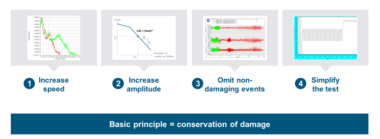
For all these methods, of course, the basic principle is to conserve the damage of the original signal or test. The damage is the most important part that you want to keep in your new, accelerated signal.
The first two methods are rather easy to apply and therefore also used frequently by many customers. But since there are limitations in how much you can accelerate your signal by using these methods and when you can safely apply them, I would like to go a little bit deeper on the last two methods.
Omit non-damaging events from long duration measurements
One of the biggest challenges when it comes to shortening real-life, long-duration measurements for durability performance validation, is to keep the damage and remove all the rest.
So, how can you remove non-damaging events from your time signal?
First a little bit of background.
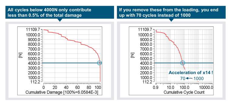
In the picture here above, you see on the left-hand side a range-pair diagram of a loading time series in a cumulative damage view. When you take a closer look, then you will see that all loading cycles below 4000N only contribute less than 0.5% of the total damage. So removing those cycles from my signal would only cause a 0,5% loss of damage compared to the original signal. 0,5% is neglectable!
If however we now express the same range pair diagram in cumulative cycle count, then we see that – if we remove all these cycles with an amplitude lower than 4000N and only keep the high-amplitude cycles – the total number of cycles goes from 1000 to 70. So by doing so, you can reduce the total time-length of the loading by more than a factor of 14, but still, keep almost the same damage!
Removing these non-damaging cycles is something that can be done automatically with the Simcenter Testlab Neo software!
Now show it with an example!
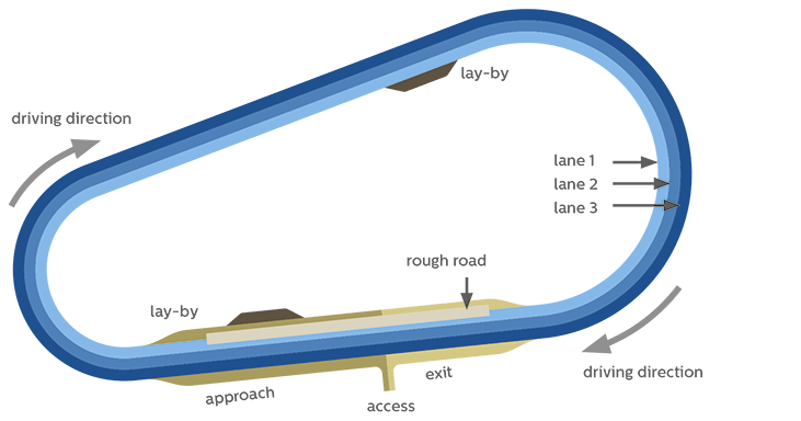
As explained in my previous blog posts, since we were only allowed to drive in one direction and not reverse after having reached the end of the durability rough road, we needed to continue each time along the oval circuit until we reached again the start of the rough road. In most cases, we stopped measuring after reaching the end of the rough road, but I have done one run where we kept on measuring while driving over the oval circuit.
The name of this measurement is called ‘Miscellaneous 02’. During the measurement, I drove 3 times over the oval circuit and rough road, so the run contains both non-damaging parts (where I drove over the oval circuit) and damaging parts (where I drove over the rough road).
This run I would like to shorten by removing the non-damaging parts and keeping only the damaging parts.
The process I prepared in Simcenter Testlab Neo to shorten the measured signal, looks like below. It looks complex, but it isn’t. The actual signal shortening is just a very small part of the process, the remainder is calculating analysis results to make comparing the result and input easy.
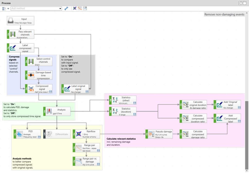
The most important part of my process is the ‘Compress signals’ part, the part marked in light blue.
- In this part of the process, I first select a couple of control channels. These are in this case all my measured strain gauges.
- Based on these control channels, I will create with the second method an index channel. In this channel the value is set to 1 for parts that contribute smaller amplitudes up to a total of 20% of the total damage. This leaves the remaining parts with a value set to 0 that totals up to 80% of the damage.
- Then based on the index channel, the next method will do the actual cutting, so it will remove those parts from the original signal which do not contribute to 80% of the total damage. In this method I also defined the fading mode to avoid transitions with steep slopes between two parts that are kept.
To better compare the compressed signals with the original signals, I extended the process to do some extra analysis on the data (like calculating statistics, damage & time duration ratio, and PSD).
After having run the process, I have with one button click a clear and compact overview of the results thanks to the ‘Pivot table’ and ‘Preview display’.
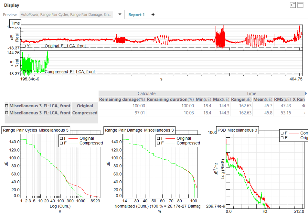
- In the upper part of the display, you see the time series. The red curve is the original signal and the green one is the compressed signal. You immediately see we compressed it quite a lot. We went from around 400 seconds to a little bit less than 21 seconds (so 90% reduction in time !).
- But despite this, if you look at the remaining damage ratios in the table in the middle, you see that the damage of both the input and compressed signal is almost the same (97%).
- In the ‘Range pair expressed in cycles’ graph, at the bottom of the display, you see that the compressed signal contains about 10 times less cycles than the original signal.
- And in the ‘Range pairs expressed in damage’ graph, you clearly see that the compressed signal is still more than 95% of the total original damage.
On the bottom right, the PSD graph is showing that although we removed quite a lot from the signal, the method did not put a lot of extra energy into the compressed signal. It also did not add frequency spikes (which could come from connecting segments after cutting) and the overall shape of the PSD remains very similar.
Creation of durability ‘Block-cycle tests’ for test benches
The signal that we created after removing the non-damaging parts, is still a rather complex signal. It contains loads with different amplitudes, different frequencies, … Many test benches are not capable of running such a signal, unfortunately. So we need to convert it into a signal with a limited number of constant amplitudes and fixed frequency. This is what we call a “block-cycle test”.
You can apply this technique if your component is rather rigid and does not use rubber or elastomer parts. Also, it works better if the loading is uniaxial.
Let me explain to you how Simcenter Testlab does it.
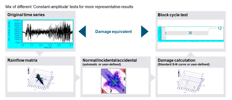
- So you start from the original time series (upper left graph)
- For this time signal, a rainflow matrix is constructed.
- Then the rainflow matrix is split up in 3 areas, representing 3 use cases of your component/vehicle.
In theory, you can choose how many amplitudes you want to have in your block-cycle test, but most of our customers take 3, to get more representative results.- A “normal” area: this area contains f.e. 90% of the original cycles and represents the normal roads (and respective loads). This area is marked with nr. 3.
- An “incidental” area: this area contains f.e. 9% of the original cycles and represents for example holes in the road. These holes can be present, but – hopefully – not very often. This is area nr. 2.
- An “accidental” area: this area finally contains f.e. 1% of the original cycles and represents for example the loads caused when hitting the curb next to the road. This happens maybe once or twice during the lifetime of the vehicle and causes very high impact (and damage) onto your vehicle. This is area nr. 1.
- For each of these 3 areas now, the maximum amplitude is taken and the mean of a sample cycle. For each of these amplitudes the damage is calculated and also the number of cycles/repetition factors in order to get the same damage for that total area.
- With these 3 amplitudes then a time signal is constructed, where each of the amplitudes is repeated in order to cause the same damage as the original signal.
This new time signal is what we call a “block cycle test”, due to the shape of the graph.
Let’s now put this into practice!
As input data, I’m going to take one of the measurements done on the Belgian block track.
In order to create a test schedule or test signal for a test bench, you typically take the signal from the displacement sensors which are mounted on the suspension of the vehicle. So in our case, I took the measured signal from the displacement sensor that was mounted on the front left wheel and the other from the front right wheel.
So here below are the two signals which I am going to simplify and convert into a block cycle test for my test bench.
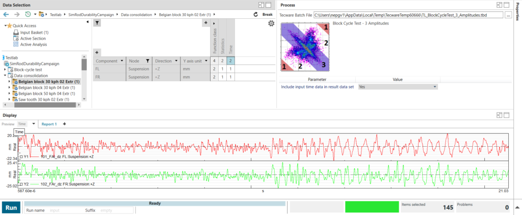
When I start the process in Simcenter Testlab Neo, I get the opportunity to further tune the parameters. If needed, I can change for example the sizes of the different areas or the frequency of the created sine wave signal. In my case, I keep the frequency at 1 hertz, but you can also set it to 4 Hz for example to accelerate even more:
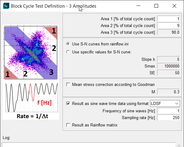
In a first step, Simcenter Testlab calculates some results:
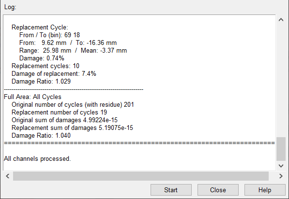
In our example, the original signal has about 200 cycles, but the simplified signal – the block cycle signal – only contains 19 cycles. But the damage ratio of the original and compressed signal is a little bit more than one, so almost the same damage.
When the process is finished and I select my first signal, you see in the ‘Preview picture’ the original signal (the green one, which I selected as input) and the actual signal for your test bench (the red one).
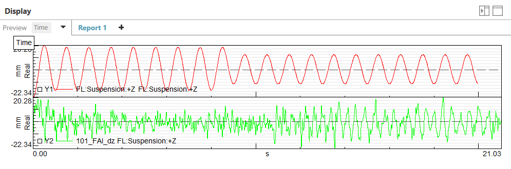
You also see the 3 amplitudes in this block cycle test signal.
These signals I can now use for my test bench schedule.
As you can see the Simcenter Testlab Neo software is so much more than just an acquisition software or data analysis tool! With Simcenter Testlab Neo you can also convert your measured data into accelerated, but damage-equivalent test schedules which can run on your test bench, and this with just a few simple clicks.
In the next blog post, I am going to elaborate a little bit more on a topic that I already touched upon in one of my previous blog posts, namely data analysis for durability. In this new blog post, I will show you how you can calculate the real fatigue lifetime of your vehicle components, by using – again – the Simcenter Testlab Neo software!
Stay tuned!
Read the other SimRod Experience blogs here: