By David Abercrombie, Mentor Graphics

Triple and quadruple patterning can baffle even the most experienced designers. David Abercrombie has some advice that can help.

As I said in Part 1 of this topic, it never ceases to amaze me how much confusion and misunderstanding there is when it comes to multi-patterning (MP) decomposition and checking. That entire first article only focused on the typical subjects I’ve had to discuss with customers regarding double-patterning (DP). I have to tell you that with the deployment of triple-patterning (TP) and quadruple-patterning (QP) at the 10nm node, the level of confusion and misunderstanding has escalated substantially. It is not surprising, I guess, as the actual software and algorithmic difficulties of TP and QP vs DP are not just linearly more difficult, but actually exponentially more difficult to solve. Given such technically difficult tool development challenges, it is not surprising that there are more difficult concepts for the foundries and designers to grasp and deal with.

At the end of the first article, I provided a summary list describing the type of expectations you should bring to DP. Those same expectations apply to TP and QP as well. But TP and QP also introduce new challenges and constraints that create additional limitations for which you must be prepared when implementing these technologies. Are you ready? Let’s dive in…

Last time, I began by describing how the layout that a designer draws is converted into a virtual graph that can be processed by the EDA tool to determine whether that layout can be legally decomposed, and if so, find a legal coloring solution. That first step remains the same for both TP and QP. In Figure 1, there is a simple set of seven polygons in the drawn layout. Spacing measurements are performed between the polygons to determine if any adjacent polygons would break the spacing constraints if they were placed on the same mask. All of the polygons that violate these spacing constraints (in this example, all seven) are then captured in a virtual graph within the EDA tool and analyzed to determine mask assignments for each polygon (or to identify the lack of a legal coloring solution). Each polygon is represented as a node in the graph, and each spacing constraint is represented as an edge in the graph.

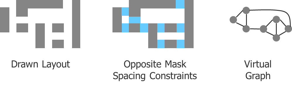
Figure 1: Translation of a layout into a virtual graph for MP analysis.

Note that the virtual graph contains no spatial information (i.e., the size or shape of the polygons, or the relative location of the polygons in space or to each other). This translation from layout to virtual graph is critical to efficiently processing the information to determine coloring. A given set of interacting polygons forming one of these graphs is called a connected component. A typical layout may form hundreds, thousands, or even millions of connected components, all independent of each other. Each connected component individually may be legally colorable or not, but a legal coloring must be found for all of them to find a legal coloring for the whole chip. So far, so good. Just like DP. However, once you try to color the graph, everything changes.

Figure 2 demonstrates a TP analysis of the virtual graph from Figure 1. Obviously, there are three color choices in TP, vs. the two color choices in DP. This would seem like a good thing on the surface, as you have more options for getting a good result. However, it is the increase in number of the options that leads to the algorithmic problems that plague a practical EDA software solution and keep you up at night.

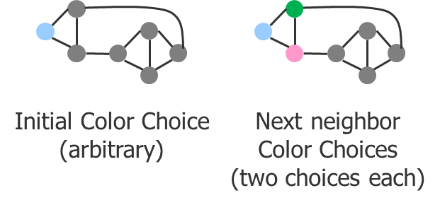
Figure 2: TP coloring analysis of a virtual graph.

In this example, I picked an arbitrary starting point (the left-most node), and one of the three color options (blue). There are two nodes connected to that original node. Each of them must be a color other than blue. There is no information at this point to help with the next color assignments, so the selection is random. I chose green for the top node, and pink for the bottom node. It turns out that there is a separator (spacing constraint) connecting these two nodes. Lucky for me, I chose two different colors for these two nodes, so they both honor the color alternation requirement from the first node, and from each other.

From those two nodes, I continue to move though the graph, coloring the next nodes as I encounter them (Figure 3). In DP, my only choice is to color the next node the opposite color of the previous node, but in TP, I have two color choices for each node I encounter, and no information as to which color to pick. By the end, I reach a point where the last two nodes connect to the blue node on the left and the pink node on the right simultaneously. Because of the separators, I only have one color choice for both of these nodes—green. But there is also a separator requirement between them, which creates a coloring error. So, does this mean that the graph is not legally colorable?

Figure 3: Arbitrary TP color selection ends in a coloring error.

In DP, yes, this result would mean that the graph is not colorable. At each step in DP, there is only one choice, so going back and trying something else is of no value. You will always end up with the same result. One pass through the nodes provides you with a conclusive answer. However, in TP, there was more than one color choice at every step until the last one, so I could have made different coloring decisions. Figure 4 shows an alternate outcome that results from changing some earlier color decisions.

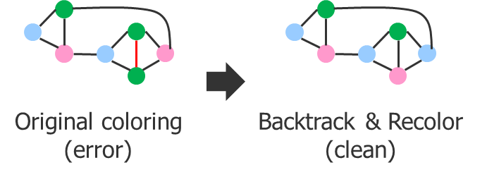
Figure 4: Alternate legal coloring solution for the virtual TP graph.

In TP, you cannot guarantee finding a correct solution with a single pass through the graph. In the worst case scenario, if only one solution existed, you might have to try every possible combination of colors to find the solution. The runtime of such an algorithm would be O(3^n) vs. the DP algorithm of O(n). Essentially, this means the runtime of DP increases linearly with more nodes in the graph, while TP and QP runtimes increase exponentially with more nodes. This is very bad news for software developers. Typical MP layouts include connected components that create graphs containing hundreds or thousands of nodes, or even more. In practical terms, the runtime would be infinite. That’s more like impractical terms. No one wants to use a software tool that runs forever.

However, let’s clear up a typical point of confusion I usually encounter here in this conversation. This does not mean that every large graph will run forever trying to find a legal coloring. In fact, a very large graph might find a coloring solution faster than a smaller graph in any given experiment. What? How? Remember that the result depends on the choices made along the way. It is possible to make “lucky” choices. You may just happen to pick a set of colors at each step that provide a correct coloring in one pass. Wow! Why don’t you just do that every time? Well, because you don’t have any way to know ahead of time what choices will work out. There is always an element of trial and error.

Algorithmically, it’s like this:

• It is quick and easy to produce a set of colors.
• It is quick and easy to determine if that set of colors is legal.

So, if your first trial produces a legal result, everything happens quickly. The problem occurs when the result of the trial is not legal. You then have to run additional trials using different decisions. Depending on how many trials it takes to find a solution, your runtime could be very long…assuming, of course, that a legal solution even exists.

Whaaat? Imagine the case where a layout does not have a legal coloring solution. How do you prove that result? The only guaranteed way to prove it is to try every coloring combination and demonstrate that they are all illegal. This technique would always require maximum runtime. If the graph of any particular connected component is large, that runtime would be practically infinite. Even if every connected component is reasonably small, if there are millions of individual connected components in the graph, then the cumulative run time could still be very long.

What’s a hard-working designer to do? Is TP and QP an intractable solution for multi-patterning? In the general case, yes, actually, it is. But by working as a team (EDA, foundry, designer), there are things we can do to make the analysis feasible for use in advanced node processes.

The first is a software trick called graph reduction. It turns out that if you look closely at any given graph component, you find that the color requirements for certain parts of the graph are trivial if other parts of the component are already colored. Let’s walk through an example.

In Figure 5, a graph component extracted from a portion of the layout is shown on the left. The graph on the right is an alternate, simpler representation of that same component. Notice that two nodes and their edges have been removed. Each of these nodes had exactly two separators going to different nodes in the larger graph. In a TP application, there are only three possible colors. Once you determine the color of the other two nodes to which one of these nodes is connected, a legal color choice for that node is guaranteed. The other nodes to which it is connected can only use up two of the possible three colors, so there will always be at least one color left to use. Graph reduction lets you remove these nodes and work on the simpler graph, knowing that once you find a solution for that graph, you can easily find a solution for the original graph.

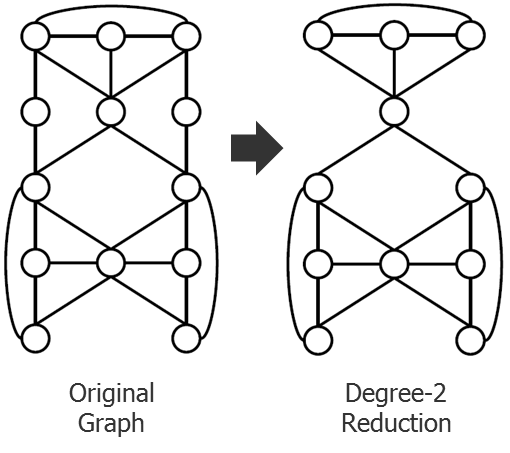
Figure 5: Degree-2 graph reduction.

Let’s take that idea a step further in Figure 6. If we look at our previous graph reduction, we now find a very interesting case of a single node in the middle that almost seems to divide the top half of the graph from the bottom half. If you duplicate this node, then split the graph into two separate graphs (as shown on the right), you can approach this problem as two separate, smaller problems. If you can find a legal coloring for the top half, and a legal coloring for the bottom half, all you have to do next is rotate the colors until the color of the duplicated node is the same. Now you can recombine the two graphs with a unified legal coloring solution. Very cool! This is called bi-connected component (BCC) articulation.

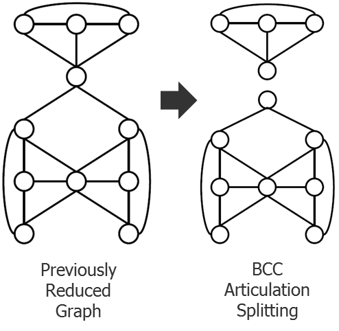
Figure 6: BCC articulation graph splitting.

Next, let’s continue combining these processes and see what happens in Figure 7. We can apply the degree-2 reduction to each of the two separate pieces from Figure 6, then apply BCC articulation splitting to those results. At this point, we’re left with three very small graph components that can no longer be reduced or split by these two techniques. These graphs are so small that even if you had to try every color combination to find a legal solution, you could do so in a reasonable runtime. Once you find a legal coloring for every one of these small graphs, you can “unwind” them back through the process of reduction and splitting to get a legal coloring for the original large graph component.

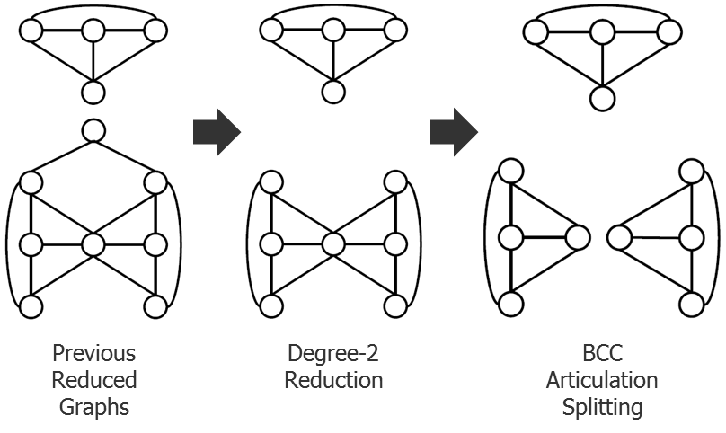
Figure 7: Reapplication of both degree-2 reduction and BCC articulation graph splitting.

Fortunately, there are algorithms with reasonable runtimes that can reduce, split, color, and unwind the results for us, meaning a connected component that may not have been originally solvable with reasonable runtime now might be. This could be our saving grace for enabling TP and QP—except you must ensure that any large graph connected component you create in a layout will be reducible into small enough sub-components. That is where teamwork comes into play.

As an EDA tool provider, Mentor has added new checking capabilities to our TP and QP tools to protect the tool from these situations that can cause extreme runtimes. This class of check is something new that designers didn’t have to deal with in DP. In DP, there were only two possible check results: clean (pass), or not colorable (fail). For the failures, various debug outputs like error and warning rings, and anchor paths were generated to help designers fix these failures.

In TP and QP, there is a third possible result, in which the coloring legality of a particular component is undetermined. Yes, you heard me: Undetermined. We call this a complexity check failure. Essentially, the tool applies all the graph reduction and splitting techniques to each component, then runs a check to see how complex the remaining sub-components are. The complexity is a function of the number of nodes left in the reduced sub-components. If the complexity is too high, then there is some probability that the sub-component could generate an impractical runtime. Again, it may not, as any particular run result is based on the “luck” of the color choices, but it could. The only robust way to guarantee designers will not encounter an excessively long runtime is to not allow that portion of layout as drawn. The tool then highlights that section of layout as a complexity failure, requiring the designer to modify it in an effort to improve how well it reduces. Figure 8 shows an example of a component that cannot be reduced further using the two graph reduction techniques.

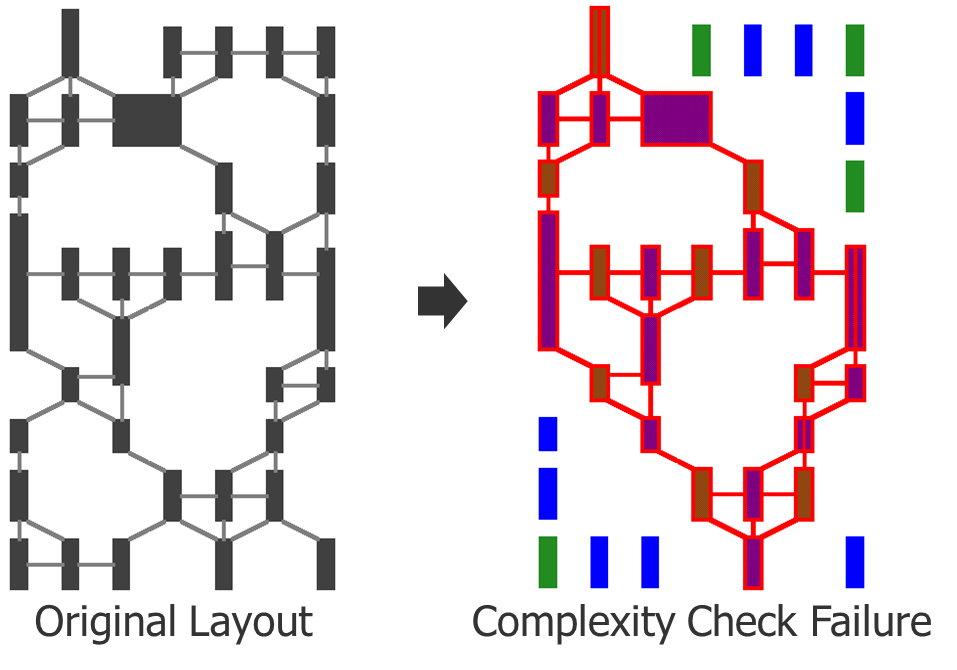
Figure 8: Complexity check failure.

The DRC rules and design methodologies for these advanced nodes must restrict the layouts that a designer creates such that the EDA graph reduction techniques can reduce the components sufficiently to make the TP/QP problem manageable algorithmically. Because some design flexibility must be sacrificed to make this process work, designers must expect some pretty hefty constraints on what they are allowed to draw in these nodes.

You may think this very strange. However, if you have ever used a router, you can probably relate to this situation. Finding a legal route for a complex layout is also a very algorithmically complex problem with potentially exponential runtime. It is easy to produce an attempted route, and easy to check if that route is legal. But it is also a trial-and-error problem. The router makes educated guesses, and if those fail, it tries alternatives. It is possible that the number of trials required to find a legal routing will require an unreasonable runtime. The only way to prove that a layout cannot be routed is to try every possible routing, which would essentially run forever. So, routers make a best effort and, if they do not achieve a solution in a given time, they give up to avoid running forever. I am sure some of you have had a router fail to find a solution, only to find a solution yourself by hand—or by suggesting the router try different options, enabling it to find a solution on the next run. The only alternative is to constrain the layout such that the number of routing trials needed would always be constrained to a reasonable number, with a check to flag layouts that are too complex to try and route. Hmmm, that sounds familiar…The problem with routing is that the constraints would be too restrictive to make it viable, so the industry has decided to live with routers that don’t always find an answer.

That is one possible approach to TP and QP. You can ignore the complexity check and hope that the tool finds a coloring solution. But in taking that approach, you have to live with the cases where it doesn’t find one. We believe that it is possible to apply reasonable DRC and design methodology constraints that would enable most designs to pass the complexity check and hence, guarantee at least a pass/fail coloring result. Even if portions of the layout fail the complexity check, we believe that designers can learn to modify those portions to solve the complexity problem, just like they have learned to modify the layout to allow routers to find a routing solution. The alternative is to color your design by hand, just like the alternative in routing is to route it by hand. There may be one-off situations where that makes sense, but in general, I believe a well-designed EDA tool, in a well-crafted use model, in the hands of an educated designer, will always provide the best overall solution.

Here is a summary of the additional expectations for TP and QP you can add to the list for DP from the last article:

• Unlike DP, the algorithmic requirements to check the decomposability of TP and QP have potential exponential run times.
• A tradeoff between significantly restricted layouts or non-deterministic automated coloring results is unavoidable.
• Expect more complex rules restricting the types of layout constructs allowed on the layers using these advanced multi-patterning techniques.
• The need to be thoroughly educated on these advanced multi-patterning techniques is higher than ever, as it will require significantly more knowledgeable layout and error debugging than prior node techniques.

I hope this helps clarify some of the more complex (no pun intended) aspects of TP and QP decomposition. In my next blog, I’ll answer some typical questions regarding designing in a full-colored flow. Particularly, weighing the pros and cons of which portions of the layout to color when to get the best efficiency in your design flow.

Author
David Abercrombie is the advanced physical verification methodology program manager at Mentor Graphics.

Liked this article? Then try this –

Article: Resetting Expectations on Multi-Patterning Decomposition and Checking – Part 1

 

This article was originally published on www.semiengineering.com