“Say your prayers” or get a rotor dynamics simulation engineer – how simulation ensures engines can survive vibrations
Engine fails at 40,000 feet
“Say your prayers” a pilot announced to passengers, after damage to the engine resulted in it becoming unbalanced, continuously shaking the entire plane. Fortunately a rotor dynamics engineer had been involved in the design.
In 2017, an Air Asia flight from Australia to Kula Lumpur had to turn around, and ground crews prepared for an emergency landing after an engine failure resulted in the entire plane vibrating, with seats shaking like a rattlesnake’s tail. Fortunately, due to the quality of engineering, the engine survived this, but how can engineers make engines that can survive such instances? We will start by introducing the basics, but there is plenty for the more engineer-minded later in this post.
An unbalanced engine is undesirable, fortunately, we can simulate the phenomenon and reduce the chance of it occurring. However, it is a complex challenge that software has only recently managed to overcome, so first we need to look at the root of the engineering problem.
An engineer’s most basic set of tools are the equations of motion. However, for these to be easily applied to a rotor mechanics problem, the object under investigation must have symmetry around its axis of rotation. To be more precise, it needs to have axisymmetry, not cyclic symmetry.
Axisymmetry vs cyclic symmetry
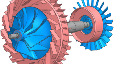
For an object to have axisymmetry, it must consist of a continuous solid around an axis, such as a spinning top. However, an object with cyclic symmetry is symmetrical around the axis but this may consist of sectors, such as the blades of a helicopter.
Generally, rotor dynamics theories rely on the axisymmetry of rotors because any data recorded by the observer of a cyclically symmetrical rotating object will show a periodic frequency as each rotor blade passes its observation point. A cyclically symmetrical object is therefore generally referred to as unsymmetrical in the field of rotor mechanics. Therefore, to understand how an unbalanced jet engine with cyclically symmetrical turbines can make the whole airplane shake, we need to consider ways of evaluating the rotor that are not the traditional external observer recording the object under observation.
Rotating vs fixed frame
By placing a measurement instrument on the axis of rotation we can measure the forces on the blade without our measurement suffering from the frequency problem. While this will give us the required values for loading on the turbine blade(s), such as centrifugal loads and Coriolis effects it creates a new problem. Since the entire airplane is not rotating around this axis, in fact it is not rotating at all, we cannot evaluate the airplane with this rotating plane but must instead study it in the inertial plane.
To compute accurate simulations of such a system that is correct with respect to theory, the simulation will need to adopt a mixed frame approach: the rotor must be computed in a rotating frame, with effects of rotations added in the equations of motion, and the stator and bearings (and the rest of the airplane) computed in a fixed frame. The developers of Simcenter 3D Rotor Dynamics and Simcenter Nastran propose that you couple such reference frames on the axis of rotation, and then offer a solution to the analysis of unsymmetric models.
Now that we know that we can model the engine and airplane together and transfer loads between them, let’s take a closer look at how we can establish critical problems originating from the engine.
Forward and backward modes in rotor dynamics
There may be numerous forces being applied to a rotating system perhaps from another rotor set within the engine or perhaps due to gyroscopic effects or structural damping. In such cases, the eigenfrequencies will get an imaginary part, as we explained in the previous blog, and the corresponding mode shapes will split into two so-called whirling modes: one rotating in the same direction as the rotor (called a forward mode), another opposite (called a backward mode).
Why use multiple harmonics and why combine a fixed and rotating frame
These whirling modes play a crucial role in rotor dynamics engineering. They are the dominant deformation patterns that will appear when phenomena occur that could lead to instability, especially at critical speeds. Therefore, for an asymmetric rotor, it raises the necessity to use multiple harmonics in a simulation. All harmonics are then superimposed linearly and recombined during postprocessing to form Orbit Plots. In an earlier blog post, we introduced the use of multiple harmonics for a system of two rotors under different unbalances, in fixed frame. Now with the release of Simcenter 3D 2406 and Simcenter Nastran 2406 it is possible to apply loads corresponding to different harmonics, in fixed or rotating reference frame, and recombine the final signal in the postprocessing. So now we can consider how forces generated by the unbalanced engine can propagate to the rest of the plane.
The airplane’s rotor was damaged, and this instability created a vibration that was then propagated through the plane. Although the vibration was disturbing, the plane was able to land without a catastrophe, so it would seem that the vibrations were not exactly the same as the natural frequency, let’s take a closer look at this considering the rotor (rotating frame) with its stator and bearings (fixed frame).
During the design phase, engineers determine the natural frequency to ensure the design avoids them as much as possible. The first step in doing this is to review the Campbell diagrams.
Critical speeds and stability of unsymmetrical models
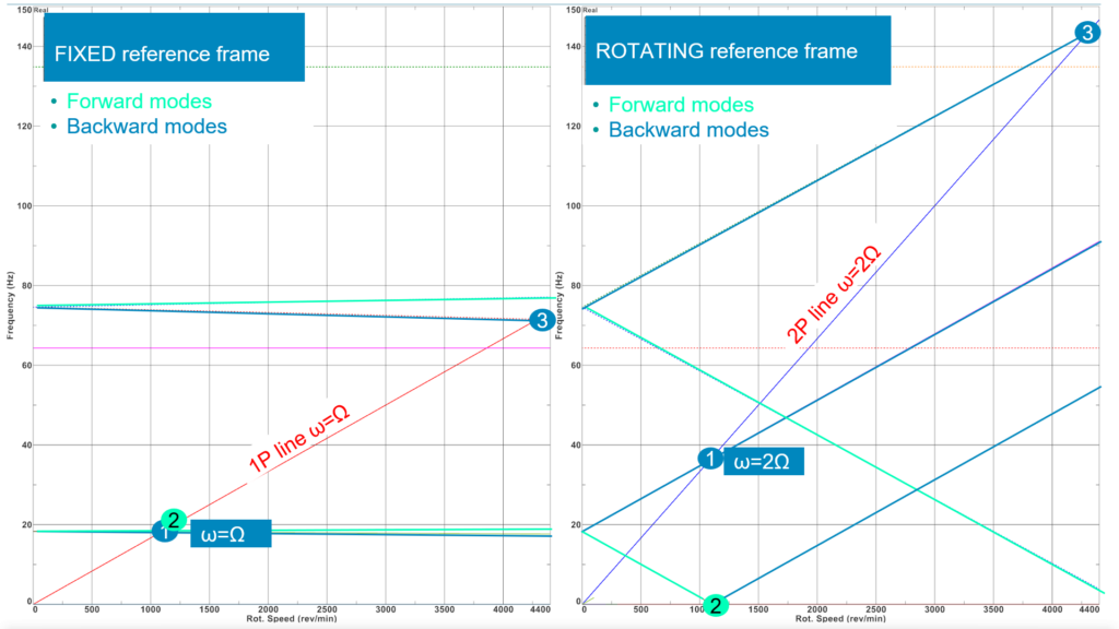
Since we are using both initial and rotating reference places we need to understand how these appear differently in the Campbell diagrams. Modes’ eigenfrequencies are represented as function of the rotation speed, their variation being a direct consequence of the gyroscopic effect. In an inertial frame, resonance occurs when the rotation speed corresponds to an eigenfrequency. We call those rotation speeds the critical speeds of the system. In a rotating reference frame, the physics is less intuitive.
On a Campbell diagram, eigenfrequencies of forward modes first decrease with the rotation speed, reach the X-axis at the critical speed (when the critical speed corresponds to a mode eigenfrequency of 0 Hz), and then increase with the rotation speed. On the same Campbell diagram, eigenfrequencies of backward modes increase with the rotation speed. Critical speeds of backward modes are found at the intersection of the line ω=2Ω, then when the rotation speed equals to half of the mode eigenfrequency (ω=2Ω).
The different interpretation of the Campbell diagram in fixed and rotating reference frames also helps us understand why a forward rotating force in the fixed frame is equivalent to a static force at 0Hz in the rotating frame, and why a backward rotating force in the rotating reference frame is equivalent to a backward rotating force at 2 Ω in the rotating reference frame.
In a rotating frame approach, the rotor can be unsymmetric (remember, cyclic symmetry does not count as symmetrical in these applications), but the stator and bearings must be isotropic. Moreover, the interpretation of Campbell diagram in a rotating frame is not straightforward. To remove these limitations, when the assembly is unsymmetric, there is an approach that is valid when the rotor has cyclic symmetry. This allows you to compute a Campbell diagram for the unsymmetric assembly, and output results in a fixed reference frame.
When the rotor is cyclic symmetrical, an unsymmetric assembly can be solved with Simcenter 3D Rotor Dynamics or Simcenter Nastran to compute the Campbell diagram, critical speeds, and stability.
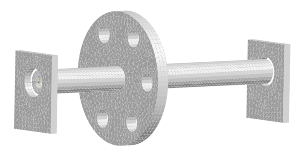
In an earlier blog post, we showed this capability on a rotor mounted on bearings, but a stator can also be added to the assembly. This capability relies on the Coleman transformation so that a cyclically symmetrical rotor can be computed in a rotating frame using time-invariant matrices and converted into a fixed frame.
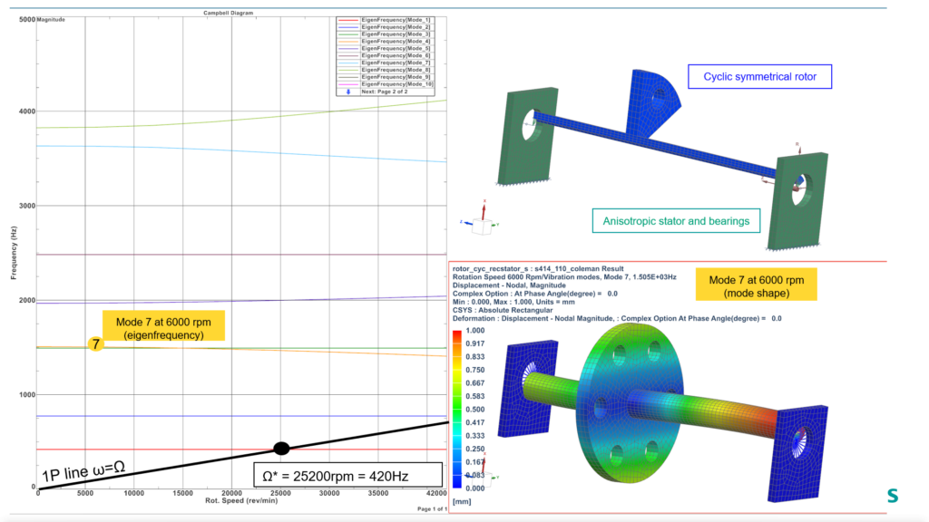
In the above picture, on the top right: assembly of the cyclic symmetric rotor, coupled to an unsymmetric stator by anisotropic bearings solved thanks to the Coleman transformation. On the bottom right, mode shape at 1500 Hz for rotation speed 6000 rpm. On the left: Campbell diagram in fixed reference frame. The critical speed of this assembly in the range [0 42,000 rpm] is found at 25,200 rpm, which corresponds to a frequency of 420 Hz.
Harmonic response of unsymmetric models
Hopefully it is now clear that a mixed frame approach can be used in the simulation of unsymmetric models, in which the rotor will be computed in the rotating reference frame, and the stator will be computed in the fixed reference frame. The coupling of both reference frames is done on the axis of rotation. We have also seen that loads are applied differently in the rotating and fixed frames: for a same load, different harmonics are used. As an extension, for vibrations computed by a harmonic response analysis, harmonic ω1=Ω will be necessary to compute the simulation in the fixed reference frame on the bearings and stator, and this harmonic will be coupled to harmonic ω0 at 0Hz and ω2 at 2Ω for the rotor computed in rotating reference frame. In cases with strong bearing anisotropy, higher harmonics are necessary. Then, when considering the rotor speed Ω as the sweeping frequency of the simulation, different coefficients [0, 1, 2, 3, …] of the Hill series will be used to describe the different harmonics.
For the equivalent model of the previous section, modeled in 3D using superelements to speed up the calculations, an unbalance has been applied at the center of the unsymmetric disk.
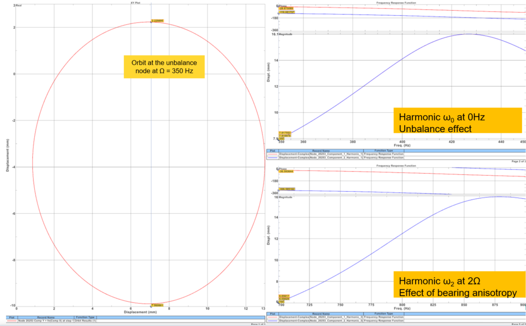
As shown in the picture below, on the right, displacement at the center of the disk is output for each harmonic separately: harmonic at 0Hz and harmonic at 2Ω. The results of the different harmonics can be recombined in the form of an orbit plot at a chosen node and at a selected frequency. In the left picture, the orbit plot is represented for the reference frequency of 350 Hz.
Harmonic ω0 at 0Hz highlights the effect of the unbalance (unbalance is a static force in the rotating reference frame). It also provides the (X,Y) coordinates of the center of the orbit. Its peak is found at about 425 Hz, which can be related to the previous simulation of the critical speeds calculation. A finer mesh would have allowed to find closer values.
Harmonic ω2 at 2Ω highlights the effects of the bearing anisotropy and corresponds to the expansion of the orbit seen on the left.
Indeed, for a system under unbalance, isotropic bearings would have provided an orbit plot reduced to a single point.
When the rotating system is totally unsymmetric, vibrations in the frequency domain can be studied in Simcenter 3D Rotor Dynamics or Simcenter Nastran for different types of rotor defects or loads, thanks to the use of multiple harmonics and a mixed frame approach.
Looking back at our airplane investigation, we can now model both the rotating parts of the engine and its fixed components such as the stator and bearings. We can also determine the complex eigenfrequencies, in both the fixed and rotating planes and then combine the results. Now, with the use of multiple harmonics along with the mixed frame approach, we can consider defects or abnormal loads. Since bird strikes on engines are not uncommon we could perhaps simulate the effect of the rotor blade being damaged in such an incident. However, the engine is not always turning at the same speed, and as the rotational speed changes the loading will change. We will also need to consider this to be sure our engine is safe.
Transient analysis of unsymmetric models
The same model can also be solved in a transient analysis. To be able to compare the results, let’s consider the same unbalance load, and reproduce the steady state behavior by defining a run up with an increasing rotation speed from 0 to 350 Hz, and then a constant rotation speed of 350 Hz.
For time-varying rotating speed or loads, the response of the rotating system is calculated by a transient analysis. A combination of superelements for the rotor in the rotating frame, stator in fixed frame, and the assembled by bearings accelerates the simulation and provides accurate results.
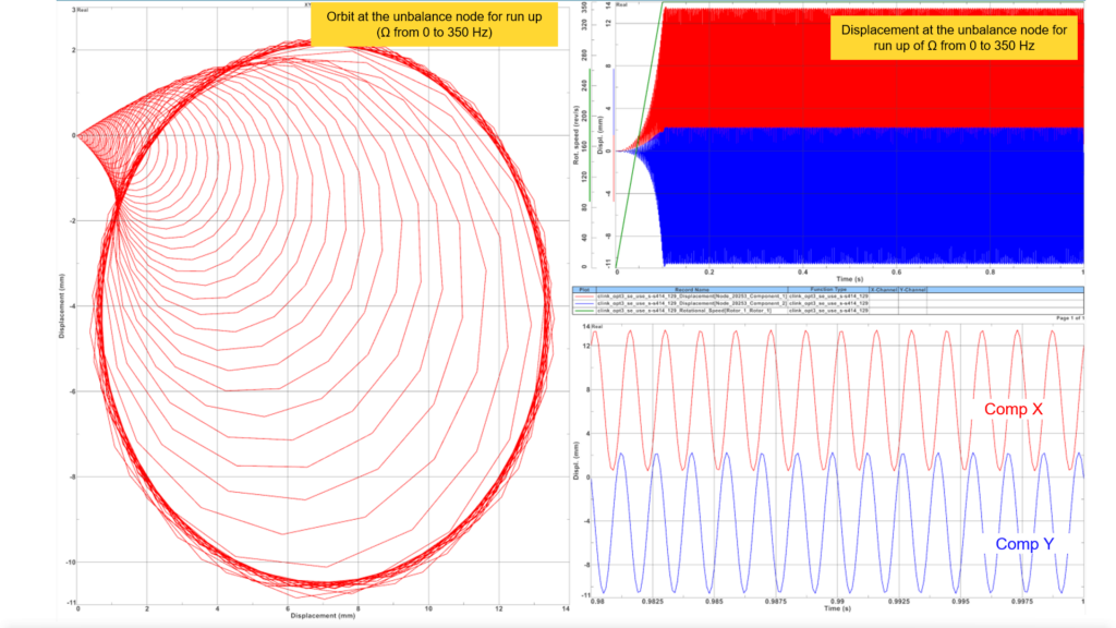
Vibrations at the center of the disk for a run-up followed by a stabilized rotation speed at 350 Hz are represented in the picture below. At that speed, the (transient) vibrations can be compared to the orbit computed in harmonic response for a steady-state simulation at a frequency of 350 Hz. We can observe that the orbit in transient for the stabilized rotation speed can be superimposed to the orbit in harmonic response when all harmonics are recombined, for that frequency of 350 Hz.
The vibration oscillates around a mean position. This mean position corresponds to the center of the orbit and corresponds to the results of harmonic at 0Hz in for the harmonic response.
Further transient analysis, for a similar steady-state scenario at a constant rotation speed, provides comparable results in the frequency response using multiple harmonics.
Conclusion
Being on an airplane when there is a mechanical malfunction is scary. However, you can take comfort in knowing the engine manufacturer and their engineers have considered many scenarios and simulated the consequences. While this was difficult in the past, new tools such as those in Simcenter 3D and Simcenter Nastran are making it easier to build models and simulate more cases, reducing the risk of possible oversights and continuing to work towards safer aircraft.
With the new capability of Simcenter 3D Rotor Dynamics and Simcenter Nastran to compute vibrations on unsymmetric rotating assemblies, the types of applications that can be solved have been expanded. Indeed, as casing and bearings are rarely isotropic, flexible rotors that are definitely not axisymmetric were left aside by rotor dynamics solutions. Now, the Campbell diagram, modified stiffened structure behavior at high rotation speeds, rotor defects like unbalance or misalignment, or any type of loads, can be studied in the time and frequency domains. In this blog post, an unsymmetric rotating assembly has been solved in complex modal analysis (rotor is cyclic symmetrical), in harmonic response, and in transient response. A complete study of an unbalance analysis was performed, and the results of the different simulations were compared together.