Demystifying Electromagnetics, Part 8 – Losses
All the energy we utilise day to day originates from the sun. The fusion processes in our local star result in ~3.828×1026 Joules of energy radiated out in all directions every second. Some of that energy hits our planet. Photosynthesized by plants that, when compressed over time, is extracted as coal, oil and gas, burned to heat water to power turbines to generate electricity to power an LCD screen that emits the photons that are entering your eyes right now.
Energy is neither created nor destroyed, it just flows. The term ‘losses’ is therefore a bit of a misnomer. Electrical and electro-magnetic systems enable the transfer of energy from a local source to something that does something useful. Not all of that input energy ends up being used for the intended purpose though. Some of it is ‘lost’, most commonly as heat.
Waste Management
There are many job roles that deal with the management of waste. From refuse collection to sewage processing, clearing up what isn’t wanted or desired is as important a role as it is unfairly maligned.
Electronics thermal management, dealing with the heating of electronic products due to the losses that occur when electrons flow, is a well-established industry supported by simulation tools such as Simcenter Flotherm. These losses cause increases in temperature leading to thermo-mechanical failures mechanisms that can result in product failure, or a required controlled derating of performance so as to limit the temperature levels.
All electronics thermal simulations require the heat dissipation as a model input, be it for a semiconductor chip, a power delivery network or any other active device. Knowing why the losses occur will help in appreciating this most important of electronics thermal simulation model inputs.
Joule Heating
We touched on Joule heating in Part 2. The voltage is a measure of the potential energy of a charge (e.g. electron) so has the units Joules per Coulomb (J/C). A flow of charges (e.g. electrons) is a current and so has the units Coulombs per second (C/s).
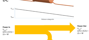
Consider a wire with current flowing through it in steady state, so no time varying behaviour, i.e. DC:
The power entering the wire is the product of the voltage (potential energy per charge) imposed at the start of the wire and the current flow rate (charges per second). Multiply the 2 together and you get J/s which is Power (W).
By the time the charges leave the wire their voltage (potential energy) has reduced but the current (charge flow rate) is the same. The power out is therefore less than the power in.
Some energy has been expended by the free electrons as they smash into all the Copper atoms, pushing out other electrons and causing the atoms to wobble. Temperature is a measure of that wobble and is the result of that used energy. This amount of energy lost to heat per second is termed ‘Joule heating’. Commonly defined as I2R.
Transient Magnetic Effects
In the above example there is a magnetic field surrounding the coil which itself holds energy. But where did this energy come from? In DC steady state there is no mention of this energy ‘loss’ required to substantiate the magnetic field. But that energy had to come from somewhere, right?
As covered in Part 4 and Part 5, the magnetic field that exists due to the current flow is instantiated as that current flow develops. The hiving-off of the energy from the electric field to generate the magnetic field delays the development of the current.
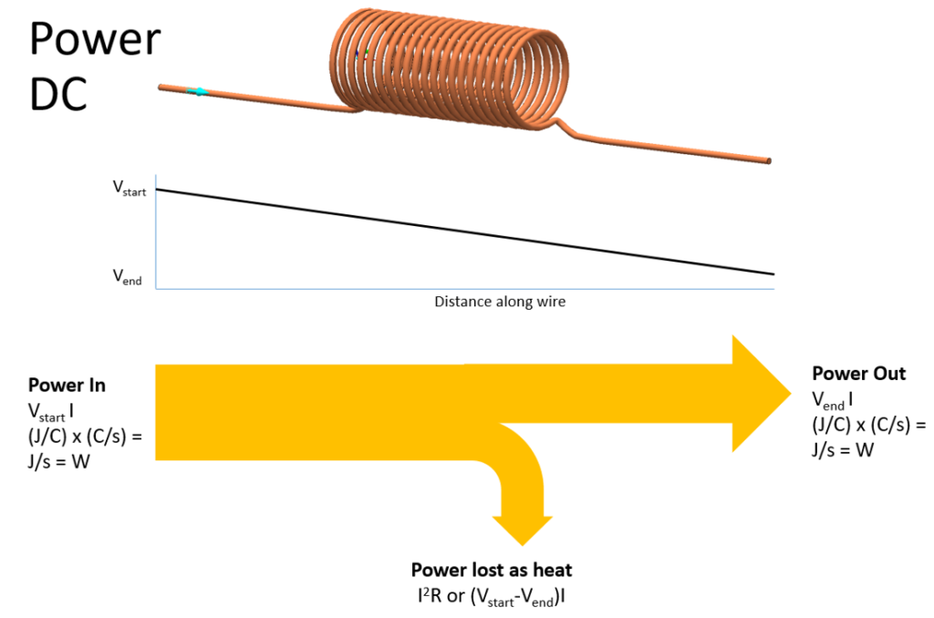
An iron core within the coil will have a magnetic field induced in it. As iron is also electrically conductive, i.e. it has free electrons, those electrons will be forced to move when they experience a changing magnetic field. Changing in space and/or time is something we’ll come back to later. So a flow of current will be induced in the core. These so called ‘eddy currents’ themselves will result in a Joule heating power loss in the core.
Going back to our coil+core Simcenter Magnet model, though this time as an axisymmetric 2D model, let’s apply a fixed voltage drop over the coils and see the transient response of the Magnetic Flux Density vectors, currents (imposed in the coil and induced in the core) and the resulting ohmic (Joule heating) losses (W/m3), until steady state:
A simple sequential description of the response would be as follows:
- After the voltage is applied across the coil, current starts to flow though the coil
- This induces a magnetic field within the core, flowing (permeating) left to right
- The magnetic field penetrates down into the center of the core over time
- The magnetic field induces an (eddy) current flowing at 90degrees to the magnetic field, in the opposite direction to the coil current that induced it
- This induced current results in Ohmic (Joule heating) losses penetrating the core
- As steady state is approached, the magnetic field does not change in time or space and so no eddy currents are induced and so no subsequent Ohmic losses occur in the core
Although it is conceptually simple to consider this sequential order of events, in reality they are all coupled and occurring concurrently.
The induced current in the core occurs where the magnetic field (rather B, the magnetic flux density) is changing either in time or space. As the Ohmic losses are related to this current squared, you can appreciate the relationship between the magnetic field, the induced currents and the resulting Ohmic heat power losses.
The magnetic field gradually penetrates the core due to the fact that once one part of the core becomes magnetised it saturates, it is not capable of being any more magnetised. So the neighbouring part of the core becomes magnetised until it also saturates and so on until the entire core is magnetised. The ‘front’ of magnetisation, as it penetrates the core, where the B field is changing rapidly in both space and time, leads to the biggest induced currents and thus biggest Ohmic losses. From a fluid dynamics analogy kind of like the turbulent kinetic energy generation being largest where the fluid velocity shear is greatest.
AC Response
Instead of applying a fixed voltage drop over the coil at t=0s and seeing the response of the system, what if a continuous sinusoidal voltage signal was imposed? The following response is after a couple of cycles where the solenoid settles down to a periodic behaviour:
In some ways much the same as the original constant voltage applied at time = 0s example. The induced current and resulting Ohmic loss front penetrates the core when there is the biggest change in coil current in time. When the voltage becomes negative over the second half of the cycle, the coil current flow direction reverses and the magnetic flux density flux vectors in the core change direction.
Regardless of this change of direction, the scalar Ohmic loss field and its penetration through the core is independent of the direction of the magnetic and induced current fields.
Hysteresis Losses
This is a bit of a weird one and commonly not a major contributor to the overall losses. As the magnetic field changes in time it reorients the atoms in the core so as to align with, and enforce, the magnetic field that passes through them. This from Part 3:
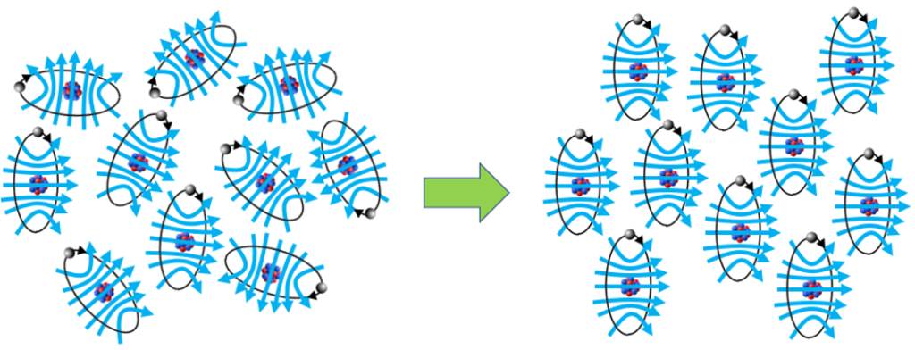
When the atoms, with their unpaired out electron, rotate so as to align themselves with the imposed magnetic field, there is an energy price to pay. Kind of like an atomic friction loss as the atoms reorientate themselves. Here’s a time averaged (over the AC cycle) of these hysteresis losses in the core:
Loss Budget
So there are 3 loss mechanisms at play; Ohmic losses in the coil, induced Ohmic losses due to eddy currents in the core, hysteresis losses in the core.
For this example there is an order of magnitude difference between these 3 loss mechanisms. Ohmic losses in the coil are ~10 times greater than the induced Ohmic losses in the core which are themselves ~10 times greater than the hysteresis losses in the core.
The losses in the coil are pure Joule heating and a function only of the current (squared) and the electrical resistance of the coil material.
The induced eddy current losses in the core are a function of the magnitude of the current in the coil, the subsequent strength of the magnetic flux density induced in the core and so the level of induced core eddy current (squared). If the frequency of change of the imposed current->induced magnetic field->induced eddy current is increased, then the time averaged eddy current losses would also increase.
These eddy currents in the core can be mitigated by lamination. Instead of having a single lump of ferromagnetic material layers of the metal are used with thin dielectric interfaces between them. The layering is normal to the direction of the eddy current, limiting its penetration and reducing the resulting eddy current I2R losses.
The hysteresis losses in the core, due to the rotational alignment of the Iron atoms to the imposed magnetic field, are a function of the rate at which the imposed magnetic field changes, i.e. the frequency at which the coil current varies, and of course the strength of that resulting induced magnetic field.
Having Fun with the dt Term
Fundamental to most of the electromagnetic physics described in this and the preceding blogs is the Lorentz force equation. Given a charge (e.g. an excess or deficit of electrons), the force a charge experiences due to it being in an electric field and/or a magnetic field:
F = q(E+(v X B))
Where E is the electric field strength, v is the velocity of the charge, B is magnetic flux density, q is the charge and F is force it experiences in Newtons.
For all these wire-wound coil solenoid examples, the electric field outside the wire is zero. There is no excess or deficiency of charges within the wire. The free electrons are just moving, the wire is net charge zero. As such. Ignoring the E field, the force that a charge would experience in a B field is just:
F = q(v X B)
In this formulation of the Lorentz equation, if the charge is moving (v is non-zero), it will experience a force on it when it passes through a magnetic field B.
Let’s break out the v term as dx/dt, a change in location over a time period:
F = q((dx X B)/dt)
The dt term is common to both the location of the charge, and the strength of the magnetic field. In this formulation, even if the charge is not moving, if the B field changes in time then a force would be exerted on the charge. It would then start to move and a moving charge is a current flow.
A moving charge in a static B field OR a static charge in a changing B field, both situations result in a force on the charge.
In the first example above, when the current reaches steady state under the imposed constant voltage drop conditions, the B field does not change in time, there are no forces exerted on the free electrons within the core, there is no induced current thus no resulting Ohmic losses.
In the second AC example, it is only when the magnetic B field changes most quickly in time (when the current flips from a +ve to -ve direction) is an induced eddy current and resulting Ohmic losses experienced in the core maximised.
Anecjoke
Einstein’s theories of relativity are astounding. To describe why you feel the same force when accelerating in a space elevator at 9.81 m/s2 as you do when standing on the surface of the earth was a milestone in human understanding.
Leaving spacetime aside, it was actually electromagnetism that Einstein was investigating when formulating his theories. Einstein’s special theory of relativity focusing on relative frames of reference is somewhat akin to the fun we had with the dt term in the preceding section. Going beyond that, the relationship between electric and magnetic fields was proved to be implicit, they are just 2 perspectives on a given charge situation dependent only on your frame of reference.
Sure, like you I find that description quite obtuse. Next time round I’m going to do a Physics degree so as to better understand Einstein’s concepts. Until then, how’s this for a bit of light entertainment:
A student recognizes Einstein on a train and asks: Excuse me, professor, but does New York stop by this train?