HPC for CFD: Superlinear scaling on supercomputers

These days, access to compute resources is just a question of budget. If you want results fast, you deploy powerful hardware. If you want cheap results, you deploy efficient hardware. If you have limited budget, you might need to wait longer.

Or at least, that is how it used to be. Nowadays, if your application supports it, you can just book compute resources on demand. You don’t have to own a HPC for CFD, you just rent it. As CFD simulations have historically been compute-intense (as they spawned from meteorology, I guess), running on different and huge compute resources is considered bare minimum requirement of these kind of applications. So when it comes to heavy duty loads, big simulations or just a huge set of design studies, you can rely on these “on demand” resources. Be it in your company’s own cluster (if you’re as lucky as I am), be it with a third-party provider.

What you pay is what you get

In these on-demand scenarios, you often face “pay per use” when looking for HPC for CFD. You use one unit for ten hours, you pay ten credits. Just the same as if you used ten units for one hour.

Naively, you could assume: splitting work on ten units will return the solution ten times as fast – exactly making up for the tenfold hourly rate. So the same solution costs the same. But as this might be true for ten units – what about one hundred? A thousand? Hundred thousand?

In CFD simulations, splitting up the simulation between different compute units is not easy. Calculating stuff is not the only thing happening. At some point (at every iteration, to be precise), the parts have to exchange data. If your CFD was a racecar aerodynamics simulation, you could think about these split up parts as equally-sized* volumes. At the edges, you have to exchange data (pressure, velocity,…) between the volumes. The effort for this exchange is not part of the calculations, it is computational overhead.

So two compute units cannot be twice as fast as a single one? You might think. It only sounds logical, because of that exchange overhead. Aktchyually, two can be MORE than twice as fast. Source: trust me. In short: the additional ultra-fast cache of the second compute unit more than compensates for the exchange overhead. When the speedup is higher than the number of additional cores, we speak of superlinear speedup.

How far can you go with HPC for CFD?

This trade-off, cache vs. exchange, when does that hold balance? And why is this question interesting to your budget?

Your budget can exploit the superlinear speedup. Just imagine, one compute unit takes ten hours for your simulation. But ten compute units are more than ten times faster, needing not just one hour, but maybe just 55 minutes. These five minutes (times ten units) you don’t have to pay, that’s your saving.

So where is the limit? When does the cluster effiency go below super-linearity? How many cores can you deploy and still benefit from superlinear speedup?

Sadly, I cannot tell you.

System 1: Some 130,048 processor cores

A joint team from Siemens and HPE ran several tests using a one-billion-cell simulation on extraordinary large compute infrastructure. The simulation is an external aerodynamics simulation of a Le Mans-like race car. 1002 million trimmed cells make up a single region symmetrical domain, which is solved with a steady coupled solver. Turbulence is modeled with a Reynolds-averaged Navier-Stokes model (K-omega SST).

The HPC for CFD in question was an HPE Cray SC EX425 with 1016 nodes, with 1000 of them used for the simulation. Each of these nodes has two AMD EPYC 7763 processors with 64 cores each. As these processors provide 256 MB L3 cache each, the total cache in the cluster is nearly half a terabyte. Per node 512 GB DDR4-3200 memory are used, with eight memory channels supported.

A quick estimate shows that even a simulation this big only uses about 2 Terabytes of memory, whereas the whole system provides more than 500 TB memory. Actually, this is only four times bigger than the L3 cache size of the whole cluster. And if you calculate it down, you notice that each processor core only works on 7800 cells of the CFD. For a HPC for CFD of that core count, a billion cell simulation gets split up into parts the size of a 2D simulation to train students in the first exercise.

Especially for these tiny partitions of one simulation, exchange speed between nodes is crucial. This task is up to the HPE Slingshot. This dragonfly topology network has up to 51.2 Tbps of bidirectional bandwidth between 64 ports. And this interconnect enabled the cluster to perform… quite well.

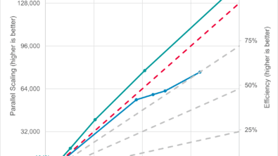
In June 2015, NCSA Blue Waters ran a simulation in Simcenter STAR-CCM+ on 102,000 cores. Up to 60,000 cores, they managed to achieve nearly 100% efficency, just scaling slightly below linear. But that is no match for HPE Cray EX with its setup: At 128,000 cores the simulation saw a speedup of 142,000 times. The baseline for these simulations was not actually a single core but 512, 4 nodes. Less would not be feasible for the 1 billion cell simulation.

Compared to just 75% efficiency at 102,000 cores in 2015 the improvements are spectacular.

But that’s not actually peak efficiency. At 32,000 cores with approximately 31,000 cells per core, the cluster reached a peak efficiency of 125%. Sounds abstract. Let me rephrase: at the correct core count you can save up to 20% simulation cost – by just using the core count with peak efficiency for your simulation.

System 2: just 32 GPUs

What if there are more options to exploit this architecture? What if you used GPUs in the cluster (on demand or on premise)?

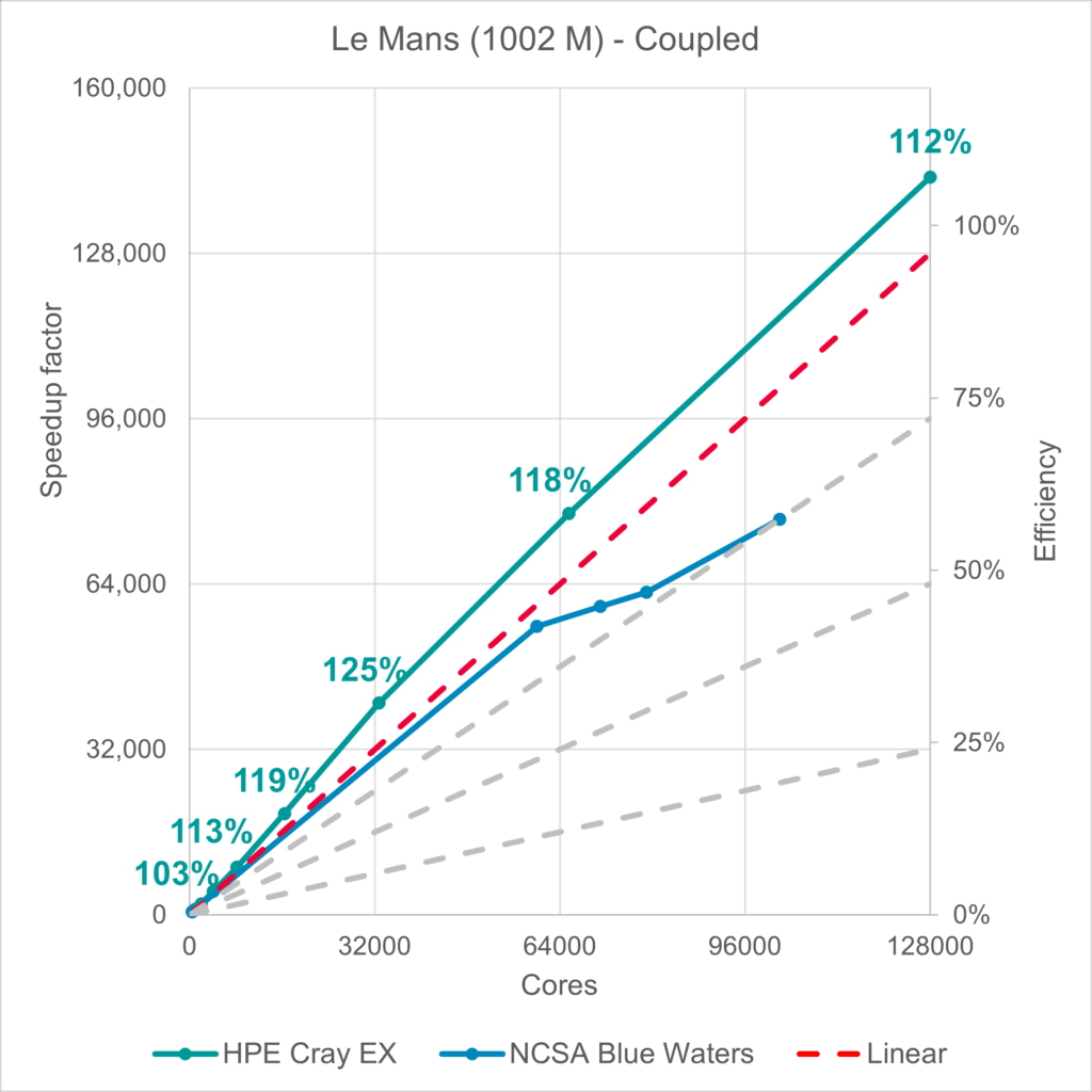
The second cluster was a HPE Cray SC EX with just 8 nodes, single CPU – but these were not directly used for the simulation. The heavy lifting was done by four AMD InstinctTM MIX250x GPUs per node, so 32 in total. For CFD, they offer 47.87 TFLOPS of FP64 floating point operations (double precision). But their real magic lies in their 128 GB HBM2e memory, with a bandwidth of 3.28 TB/s.

Exploiting this memory, CFD software becomes incredibly efficient, so that the 8 nodes with 4 GPUs each were 9.8 times faster than 8 nodes of system 1, with each 2x 64 CPU cores.

But “faster” is no longer a real criterion, if you can just scale up beyond 8 nodes, beyond 1024 processor cores. So let us put it into perspective: 32 GPUs are as fast as 10035 CPU cores. One GPU is as fast as 314 CPU cores. One GPU is nearly as fast as three CPU nodes.

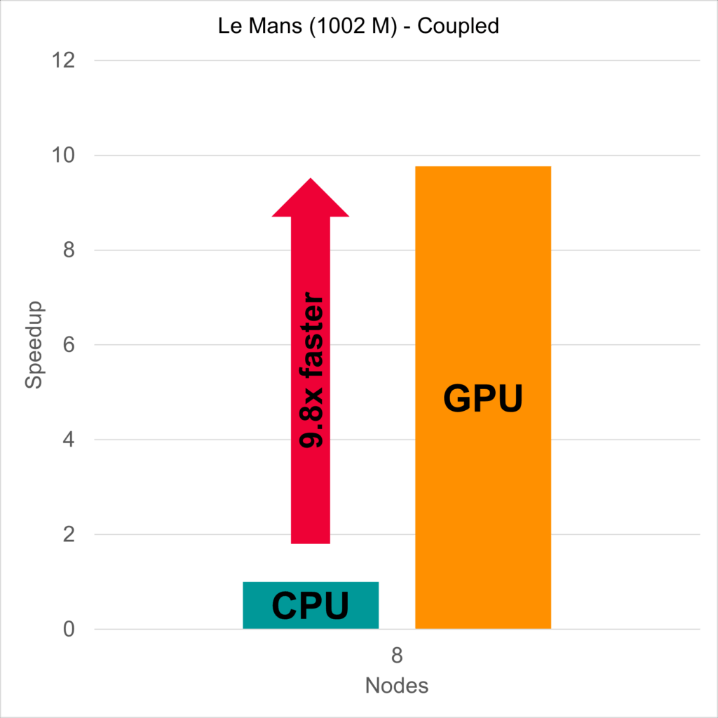
One of the most important aspects for simulation cost is energy consumption – and here is the real strength of GPUs. When you compare the energy consumption of 8 GPU nodes to 8 CPU nodes while simulating said 1 billion cell racecar – the GPU nodes consume 55% less energy for the whole simulation.

Conclusion for HPC for CFD

To achieve fast and efficient simulation results, some checkboxes must be ticked:

• Fast data exchange in compute units, e.g. high memory transfer rates.
• Fast data exchange between compute units, e.g. high speed interconnect topology.
• Simulation code that scales well, even when breaking up simulations into tiny pieces.

Respecting and optimizing these, simulations can run cheaper and more efficient. Knowing the simulation and the respective systems can also lead to a cost decrease by exploiting super-linear speedup. Changing to GPU platforms can furthermore reduce the energy consumption for the same simulation with consistent results.

Read it fully here: HPE Whitepaper

____________________

* ideally, equal computational effort. But maybe, we can assume same cell count for a start. Maybe redistribute, re-partition later, if the code notices different runtime between partitions.