Bayesian Focusing: allrounder for localization and quantification of sound sources
Bayesian Focusing is a microphone array method for sound source localization. It outperforms traditional methods both in sound source localization and quantification. It covers the full frequency range and allows a wider distance to the source compared to traditional methods. It works both for correlated and uncorrelated sources, contrary to other wide-band methods.
That makes this method an allrounder in its kind. But what is this method, and how does it work?
Before explaining that, let’s first have a closer look into how microphone array-based sound source localization methods emerged. And how their disadvantages have boosted development of methods over the years.
Holography – the old way
Nearfield Acoustic Holography (NAH) is one of the oldest known microphone-array-based method for Sound Source Localization (SSL). It can still be considered as the reference for an industrialized SSL solution, being available now for more than 30 years.
NAH requires a rectangular microphone array where all microphones are spaced at the same distance. It still has the best spatial resolution known today, which is the ability to separate two closely spaced sound sources. To be precise, the spatial resolution is equal to the spacing between two microphones, for the entire applicable frequency range. Additionally, the frequency range of NAH is bounded on the lower end by the size of array, and on the upper end again by the spacing between the microphones. More precisely: the spacing of the microphones is half the wavelength of the maximum frequency, and the width of the array is the wavelength of the minimum frequency. Furthermore, the array needs to cover the entire object. Finally, it is a nearfield method. It takes advantage not only of propagating waves, but also of so-called evanescent waves. These are sound waves that do not propagate, exist only for several wavelengths away from the source, and then vanish.
Practically that means that if you want to measure sound sources on an object over a range of 340Hz to 3400Hz, you would need an array of 1m by 1m (to cover the minimum of 340Hz), with a microphone spacing of 5cm (half the wavelength of 3400Hz, or 10cm). That leads to an array of 21×21 = 441 microphones, and the measurements should be done at about 5-10cm distance. Often it is also not practical to measure at 5-10cm distance as the object itself is not flat. Or there are cables, tubes etc. running out of the object. In practice that means that NAH is typically measured in patches with smaller square or line arrays that are combined afterwards. That makes this a huge measurement task. But if you are prepared to take the effort, then the result is rewarding.
Modern array solutions boost new method development
These impracticalities have shifted focus to beamforming. Beamforming, or sum-and-delay in its simplest form, gives best results with circular arrays with irregularly spaced microphones. This can be fully random, with spirals, or star line arrays. For beamforming all data can typically be measured at once. Beamforming also has the great property that it can localize sources outside the boundaries of the array. Therefore it does not need that many microphones.
Beamforming arrays needs to measure in the farfield as they assume planar sound waves. This is not true in reality of course, but if sufficiently far away from the source then this assumption holds. The farfield is typically defined as further away than the diameter of the array.
Beamforming has a spatial resolution proportional to the wavelength λ, multiplied with the ratio between the distance d to the source and the diameter D of the array: λ∙d/D. That means that beamforming gives good results in high frequency and reasonable results on mid frequency. But in low frequency results are not usable, typically below 500-2000Hz depending on the size of the array. As an example, a beamforming results at 340Hz would put a red spot on the map with a diameter of 1m.
Addressing the convenience of getting a fast, acoustic snapshot to localize sound sources, a lot of development has been done over the past 20 years to improve beamforming results in low frequency:
- Nearfield Focalization allowed to improve the spatial resolution with a factor 2, by taking spherical waves into account while also moving the array into the nearfield
- NAH was reformulated to work also with irregular microphones arrays, boosting performance in the range 100Hz-1000Hz
- Deconvolution methods aim at inversing the convolution of the array with the sound sources
- Inverse methods that reconstruct the sound sources by considering the microphone measurements and a priori knowledge on the propagation of sound towards the microphones. Bayesian focusing is one such inverse method.
- Some of these methods also provide quantification of the sources, allowing to rank source according to their partial sound power contribution.
Next to that, several trends have emerged on hardware as well:
- Computing power has evolved such that beamforming results can be calculated in real-time.
- Analog microphones are being replaced by much cheaper digital MEMS microphones allowing many more microphones on the same array area.
What is Bayesian Focusing and why does it outperform other methods?
Bayesian Focusing is an inverse method for sound source localization. It solves the inverse problem in a specific way. In general, the inverse problem is defined as p=Gq+b, where p are the sound pressure measurements of all the microphones, G is the transfer function matrix of how the sound propagates from each possible source point to all microphones on the array, q are the sound sources strengths (volume velocities) that we are trying to identify, and b is a residual term.
The elegant way in which Bayesian Focusing solves the inverse problem is to define it as a probabilistic problem. It assesses, according to a Gaussian probability density function, the probability that a certain point on the source map actually contains a real source, given the microphone input and propagating transfer functions.
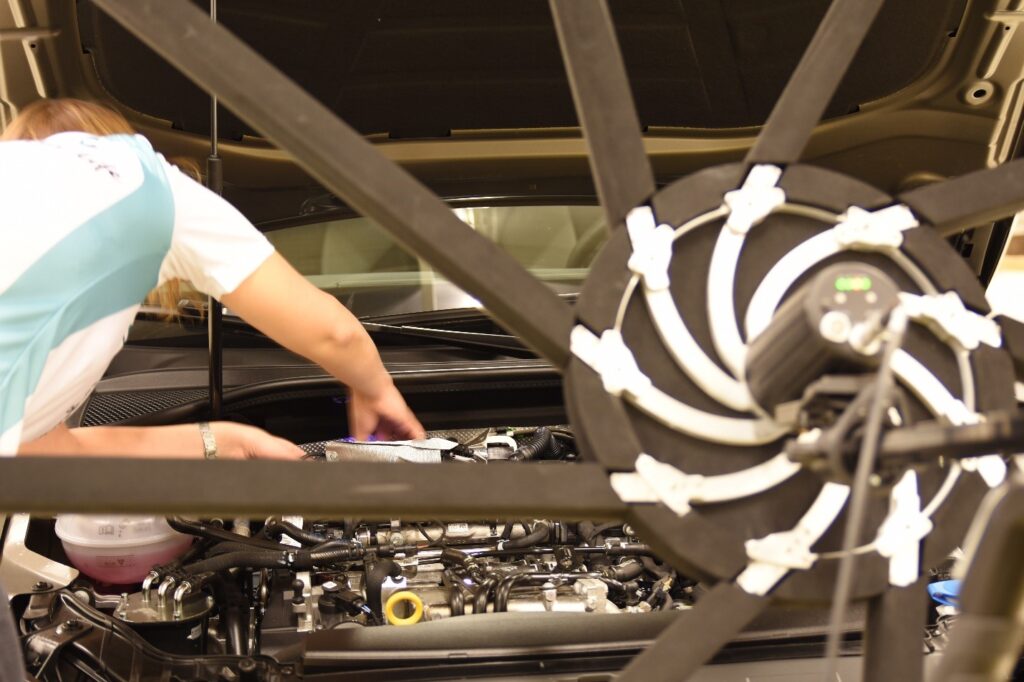
In order to solve the mentioned inverse problem, most of the methods are based on the decomposition of the sound pressure field on a spatial basis, such as plane wave basis for NAH. Bayesian Focusing has shown that it can actually adapt to a so-called optimal spatial base. That means that it can get similarly good results to problems that are known to be optimal for other methods. As an example, we saw that NAH works well when all sources are in the same plane. Bayesian Focusing would get similar results as NAH on such 2D plane, but also if the sources would all not be in the same plane. Figure 1 shows a comparison of how Bayesian Focusing improves beamforming results. The source is a small speaker playing white noise. This example focuses on the low frequency 3rd octave bands with center frequencies 200Hz, 250Hz, and 315Hz. The dynamic range is 8dB, meaning that in a real case also secondary lower level sources can be localized.
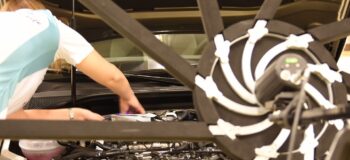
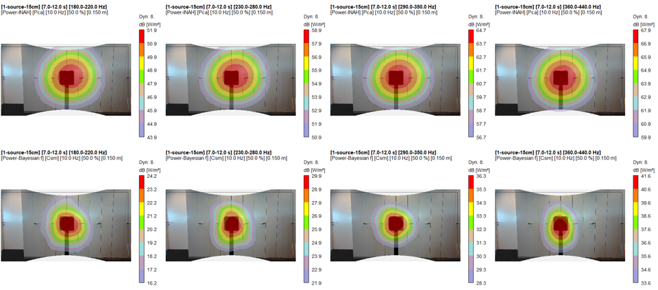
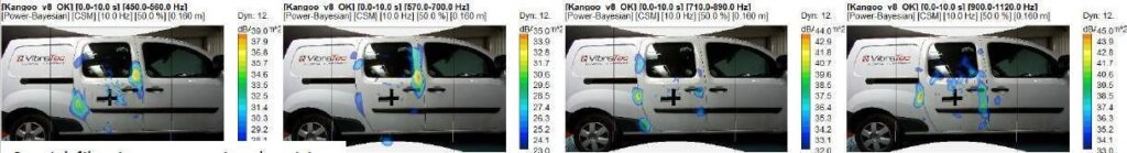
Figure 2 shows a comparison of Bayesian Focusing against iNAH on an air intake line on a vehicle in a chassis dynamometer test bench. At a measurement distance of 23cm Bayesian focusing performs quite well, especially at 500Hz and 630Hz. For iNAH, 23cm is not yet the optimal analysis distance which would be 10-14cm. But in a practical case it is not always possible to reach that distance with a microphone array.
As most inverse methods for sound source localization, Bayesian Focusing has two intrinsic sensitivities that pop up when applying this method on real cases. The first one is the sensitivity to exterior noise. As an inverse method, the assumption is made that all the measured noise is generated by sources that are located on the calculation grid. Each intersection on the grid can be a source point. So, if a sound source is located outside of the calculation grid, all that energy will be reconstructed on the grid. The second sensitivity that all inverse methods are sensitive to is the scattering effect of the array, where sound scatters on the array structure and microphones themselves. This is more penalizing in configurations with extremely non-centered sources that are spread all around the calculation grid, and in very complex environments that reverberate the sound.
Both the external noise and the scattering effect are be removed by applying advanced filtering techniques. With these sensitivities addressed, Bayesian Focusing can be applied as an industrial method.
Without going into further detail here (see ref. 1 & 2 below for a comprehensive overview) Bayesian Focusing has proven to be an accurate sound source localization and quantitfication method that significantly improves spatial resolution especially in low frequency. It has more flexibility to measurement distance when compared with NAH, and contrary to Deconvolution methods it has the ability to reconstruct correlated sources as well.
Is Bayesian Focusing an alternative to Nearfield Acoustic Holography?
To answer that question, we have to look at 2 criteria: the quality of localization & quantification, and the practical usability of the solution.
First, the quality of localization: industrial benchmarks have shown that the quality of localization is similar or better compared to NAH, both in terms of dynamic range as well as in spatial resolution. As an example, Figure 3 shows the perfect case for NAH: it’s an acoustic transparency application, where the source plane is almost flat.
Inside the van there are 4 volume velocity sources all generating an uncorrelated white noise sound field. This creates a pressure field inside the cavity of the van that is diffuse enough to be used for the transparency test. On the outside a NAH array measurement is done at a distance of 12cm. In this case the array consisted of 2 vertical line arrays of 14 microphones, with a microphone spacing of 6cm. To get to the required spacing of 3 cm (expected maximum frequency < 6kHz), and to cover the entire side panel of the van, the array is put at 168 unique locations. That means more than 4700 individual microphone measurements are used.
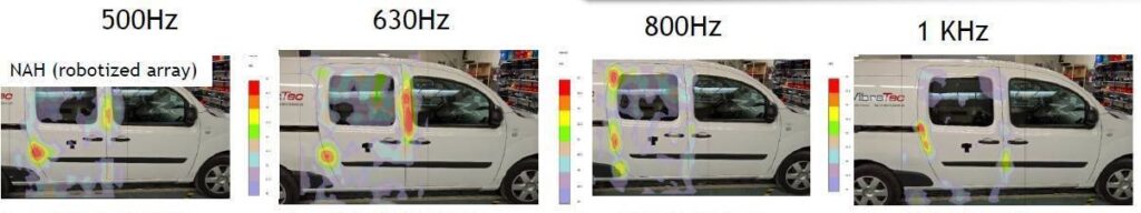
Coming back to Figure 3, the top row shows the NAH results, and the bottom row shows the Bayesian Focusing results. All the results are presented with a 12dB display dynamic. By comparing the holograms, it can be seen that there is a very good match. Spatial resolution can be considered equal, while the dynamic range is even a bit better.
Next to localizing sources over the entire frequency range, also the quality of quantification was also assessed in the benchmark. It was found to be correct with the same precision as NAH, when directly comparing with Sound Intensity as a reference.
Next, from the usability point of view, NAH required the measurement of 4704 measurement locations. To make that manageable, a robot pilots the array to all these positions. At each position a measurement is automatically taken. The scan itself took 40 minutes for a single measurement condition, while the entire setup, setting up the data management, double-checking the measurement position took more than half a day for an experienced measurement crew. After that, all data has to be combined and processed by the NAH tool, a task that can easily take the rest of the day.
When comparing that to Bayesian Focusing we used a Simcenter Sound Camera Digital Array with 9 arms and 117 digital MEMS microphones in total, and a diameter of 1.50m. Setup took 5mins, multiple measurements were done for different conditions, all in less than 15 minutes. A first series of results can be available within half an hour, for multiple measurement conditions. Modifications on the source side can be done long and assessed for effectiveness long before the NAH results become available. Additionally, as all data is acquired in a single measurement, semi-stationary or even slow transient source conditions are not an obstacle.
So, to answer the question at the beginning of this section: Yes, Bayesian Focusing can replace NAH as it has equal or better localization and quantification results, and it increases the efficiency from measurement to result by a factor 5-10.
Conclusion
Bayesian Focusing for sound source localization is a quantitative method covering the full frequency range and has a wider distance applicability compared to conventional Nearfield Acoustic Holography techniques. It gives good results both for correlated and uncorrelated sources, contrary to other wide frequency band methods. Next, it works for further distances, up to the array diameter, which is more practical for complex test objects. It has a spatial resolution equal to Nearfield Acoustic Holography in low frequency, and better in mid frequency. The quantitative results show an accurate sound power within +/- 2dB over the full frequency range, for distances up to the array size. Finally, engineers can be much more efficient, up to a factor 5 to 10, allowing several design modifications to be tested while the test object is still available.
It can then therefore be stated that in cases where fast beamforming methods do not give the requested quality, Bayesian Focusing should be used. It outperforms other methods in the nearfield, mid distance field, and farfield. Both for localization and quantification, and for correlated and uncorrelated sources.
It’s the allrounder of sound source localization methods, and is available in the Simcenter Testlab HD Acoustic Camera product family.
Are you looking for more information to understand the latest Sound Source Localization methods? Have a look here.
Interested to see how customers use Sound Source Localization in practice? Read this blog.
Discover the full Simcenter Testlab acoustic product suite here.
References:
- Antoni, J. (2012). A Bayesian approach to sound source reconstruction: Optimal basis, regularization, and focusing. The Journal of the Acoustical Society of America, 131, 2873-2890. doi:10.1121/1.3685484
- Le Magueresse, T. (2016). Multidimensional unified approach of the inverse problem of acoustic identification. Lyon: INSA Lyon