Qsources: Q-MED frequency response curve applied to acoustic FRF
In this blog post, learn more about the calibration factsheet provided with calibration service of the Simcenter Qsources Exciters. In detail the Low Frequency Monopole (Q-MED).
What is a calibration certificate?
The calibration certificate of Qsources reports the averaged RMS calibration value for the frequency range specified. The final user needs this value to perform FRF measurements. Figure 1 below reports an example of a calibration certificate for Qsources noise source Q-MED. The Q-MED source has an RMS sensitivity of -8.92E+04 V/m3 averaged over the frequency range 20-500 Hz. The same certificate also reports the frequency response curve of the instrument in dB scale. The reference to obtain the dB value is the sensitivity in the same spreadsheet -8.92E+04 V/m3. The frequency response curve graphic in Figure 1 shows the one-third octave band values in dB scale. While the calibration spreadsheet in the Excel table in Figure 2 reports linear sensitivity values in one-third octave bands. The frequency response curve of the Q-MED shows that the instrument sensitivity has mainly a flat trend in frequency domain. However, the sensitivity response curve of Qsources can be useful to obtain a more precise FRF amplitude as explained later.
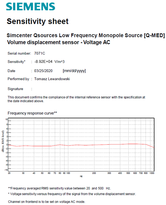
Figure 1 Example of calibration spreadsheet.
The Excel table below (attached to the calibration factsheet) reports the sensitivity values for the Q-MED in one-third octave bands. The dB value in Figure 1 is obtained from the sensitivity value in the one-third octave band and averaged RMS sensitivity as the dB reference (Figure 2).
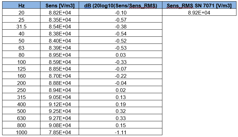
Figure 2 Calculation of Frequency Response Function of the instrument.
Integration of FRF of calibration factsheet into FRF measurements
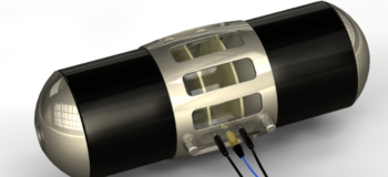
With Q-MED the user can perform an acoustic FRF measurement with noise source and microphone. The user enters the constant Q-MED RMS sensitivity value in Testlab channel setup.
However, for example, the Q-MED instrument sensitivity at 20 Hz has a value of 8.82E+04 V/m3 instead of the average value entered during measurement setup of 8.92E+04 V/m3 (see Figure 2). This little difference can deal with slightly variation in resulting FRF measure. If a user focuses in a behavior of FRF at 20 Hz he/she can correct the measured value. Following this process the 20 Hz FRF result is more precise due to the corrected sensitivity applied for different frequencies. In Testlab Channel Setup, the user enters the Q-MED RMS sensitivity value. However, the user can correct the FRF spectral values after performing the measurement. This is possible using a post processing calculation to account for the variation of source sensitivity over the frequency range. The sensitivity values are helpful to correct the amplitude.
The acoustic FRF measurement results can be corrected in amplitude using the FRF of Q-MED in one-third octave bands present in the calibration certificate.
Figure 3 displays an example of an acoustic FRF done with a Q-MED noise source.
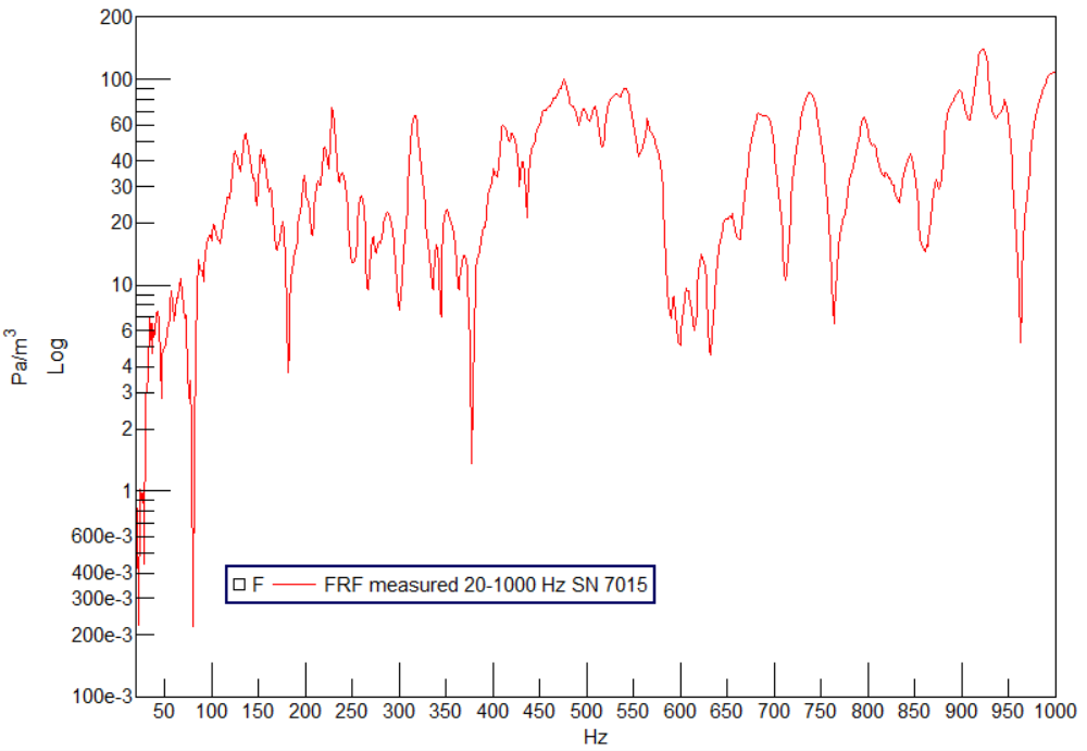
Figure 3 FRF measured between Q-MED and microphone.
The FRF of Figure 3 shows an example of a measured acoustic FRF in narrowband format. This will be compared with the Q-MED instrument Frequency Response Function in one-third octave bands.
The measured FRF of the example in Figure 3 was obtained with noise source Q-MED Serial Number 7015. Figure 4 reports the calibration sheet of Q-MED Serial Number 7015.
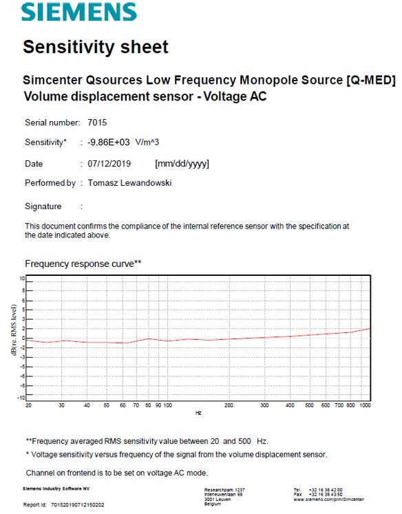
Figure 4 Calibration factsheet of Q-MED noise source.
The frequency response function of the instrument V/m3 reported below in Figure 5 shall be converted to narrowband values to be compared with the measured FRF in Figure 3.
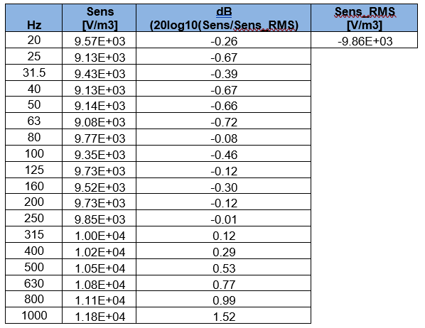
Figure 5 Calculation in dB of Q-MED frequency response function.
The relation to obtain the corrected FRF measured value starting from the Q-MED sensitivity curve and the Q-MED RMS sensitivity value is explained hereafter:
- FRFcorrected is the corrected FRF result;
- Lcorrected is the corrected FRF level result in dB;
- senscorr is the frequency dependent actual sensitivity;
- sensRMS is the average RMS sensitivity over the frequency 20-500 Hz of the calibration factsheet.
The user shall interpolate the one-third octave band Q-MED FRF curve to multiply this with the narrowband Acoustic FRF in Testlab MIMO FRF.
To perform the interpolation, it is necessary to use the Testlab MIMO FRF Testing Add-in named Data Block Editor as shown in Figure 6.
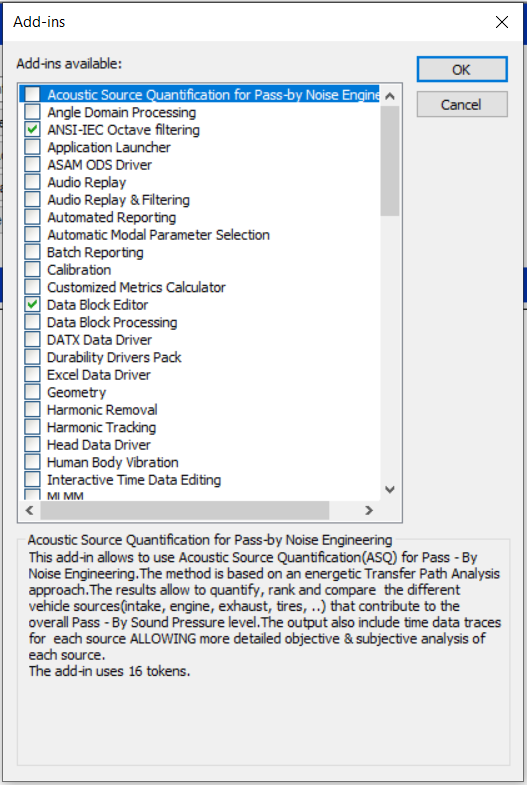
Figure 6 TestLab MIMO FRF Testing Block Editor add in.
The Frequency Response Function of the Q-MED shall be inserted in the Data Block Editor in one-third octave band format first (Figure 7). Then the user shall convert in narrowband (same frequency lines as the acoustic measured FRF) with the interpolation method (Figure 8).
The interpolation is done by clicking update after changing the number of lines and the fixed frequency increment to match those parameters of the measured FRF.
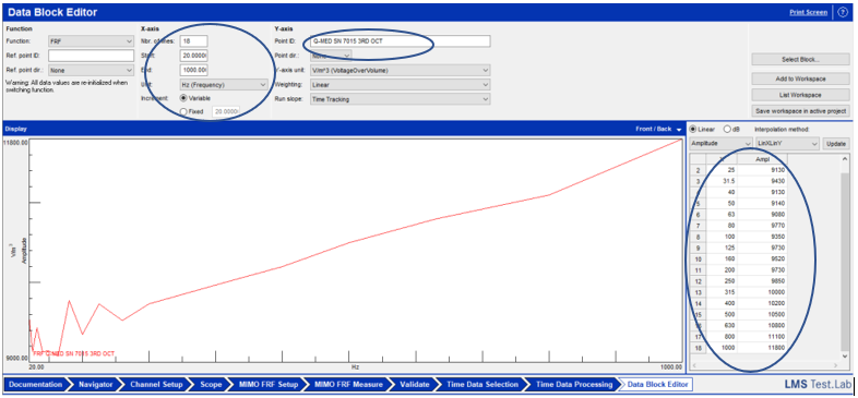
Figure 7 Q-MED FRF inserted as one-third octave band spectrum in Data Block Editor.
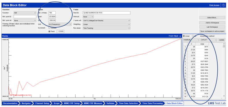
Figure 8 Q-MED FRF converted to narrowband with the linear interpolation method.
As highlighted in Figure 7 and in Figure 8, the Q-MED FRF has V/m^3 unit. If this unit is not automatically present in the Data Block Editor Y-axis units, the user shall add it in Simcenter Configuration and Unit System 2.2 or latest version 3.0 as shown in Figure 9.
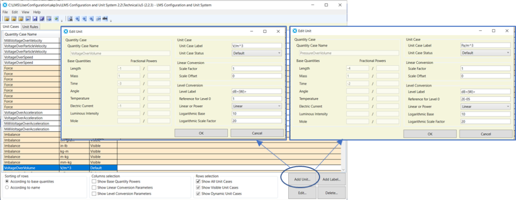
Figure 9 LMS Configuration and Unit System.
The user shall save the interpolated Q-MED narrowband FRF curve in the active workspace.
After that, the user shall import the following spectra into Data Calculator:
- the narrowband measured Acoustic FRF;
- the Q-MED FRF interpolated to narrowband;
- the spectrum of the average RMS sensitivity (constant amplitude over frequency).
Figure 10 shows how to create the spectrum of the average RMS sensitivity of Qsources in Data Block Editor.
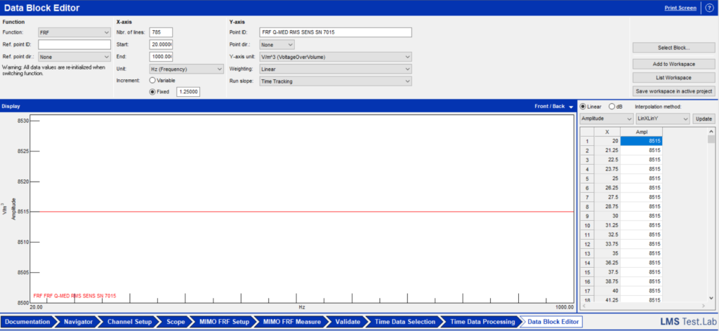
Figure 10 Average RMS sensitivity creation in Data Block Editor.
With all of these spectra having the same bandwidth and the same frequency resolution, it is possible to calculate the corrected Acoustic FRF by multiplying the measured Acoustic FRF with the Q-MED FRF and dividing by the Sensitivity RMS value, as shown in Figure 11 and Figure 12.
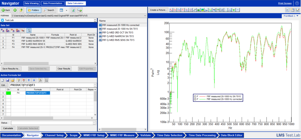
Figure 11 Calculation of corrected FRF in Navigator, Data Calculator.
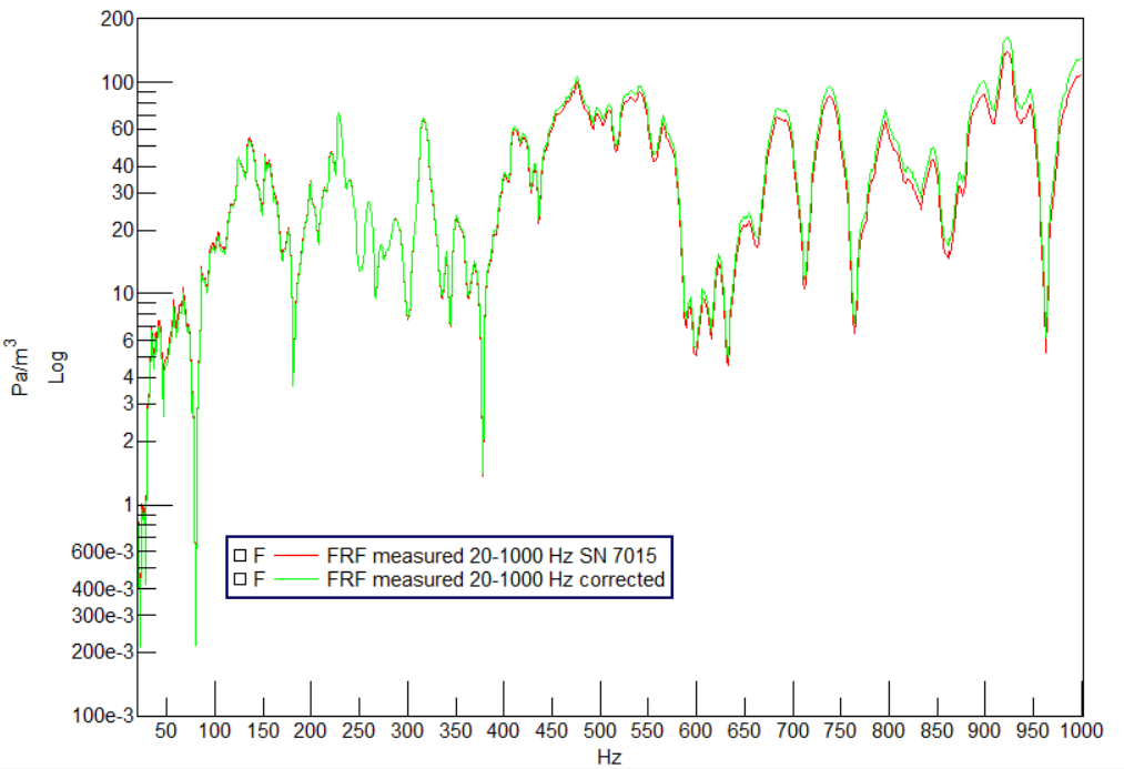
Figure 12 Calculation of the corrected Acoustic FRF (green curve).
As shown in Figure 12 at low frequencies the corrected FRF curve has lower values compared to the uncorrected one.
While for middle frequencies the curves overlap and for high frequencies the corrected FRF (green curve) has significant higher values. This trend is due to the application of Qsources Q-MED calibration curve. If the range of interest for the user is low or high frequencies it is reasonable to perform this procedure to obtain more precise measured FRF values.
In conclusion, the user can make use of these corrected values for further analysis or comparison to avoid the influence of the source on the measured FRF.


