Acoustic Simulation: Listen to the music, not the noise
Ever since Gordon Moore, the co-founder of Intel, postulated the law named after him about the doubling of the number of transistors every two years, there have been dramatic improvements in the computational capabilities of electronic devices. The reduction in size of components coupled with the increased demand for computational power has resulted in ever higher power densities requiring optimized and advanced cooling configurations to maintain a safe operating temperature. Electronics thermal management is a separate topic and beyond the scope of this blog. However, I would like to discuss one of the consequences of increased electronic performance – noise!
Anyone working during the summer in an office is no doubt accustomed to the fans of their computers or laptops spinning up when the number of applications running in parallel is increased, or even more fun, one starts running an advanced Computational Fluid Dynamics (CFD) or Finite Element Method (FEM) simulation. Fan noise, while simply thought of as an unavoidable inconvenience, is the result of a complex interaction between the fan itself and the airflow it generates. For this reason, it can be sometimes referred to as flow-induced noise or aero-acoustics.
Notwithstanding the need to properly cool all these electronic components in the cramped package space of a modern laptop, people have come to expect the noise it generates to be unintrusive. Noise-cancelling headphones can help you out here, but they are far from the ideal solution during a hot summer day. Moreover, the acoustic performance has become one of the foremost indicators of high-quality laptop brands – combining the gentle hum of the fans with a clear, vibrant, and well-placed set of speakers playing your favorite tunes.
This puts a lot of pressure on the engineers developing these systems. Let’s find out how state-of-the-art acoustic simulation tools can help dedicated engineers predict acoustic performance earlier, faster, and more reliably.
The unavoidable “bad” sound…
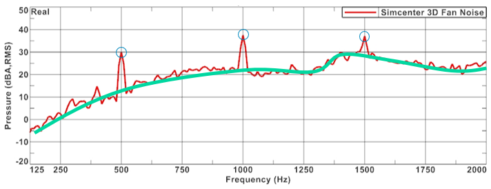
When analyzing the noise signature of a fan there are typically two components, tonal and broadband noise, as shown in Figure 1. Tones can be clearly visible as higher sound pressure levels resulting from periodic interactions of the incoming air with the fan’s blades (blue circles). The broadband noise component is caused by random loading forces on the blades which can be induced by things like ingestion of turbulence or boundary layer development (green line).
Considering that fan noise is the result of the interaction between aerodynamic flow and acoustic wave propagation, both the airflow and the acoustics need to be simulated. Acoustic wave propagation can be directly included in a CFD simulation already used to assess the cooling performance of the design but this – while possible – can present significant challenges. These challenges are mainly caused by the significant differences in length scales between the acoustic waves and the flow. This means that high order physics schemes and exceptionally long calculation times are required so this approach is not always feasible.
Hybrid approaches have been developed in response to this, in which the generation and propagation of the sound is separated. CFD data is used to reconstruct the sound sources due to flow effects, while acoustic simulation models are used to propagate the sound waves caused by these sources. This offers the advantage of allowing more efficient low-order flow simulations and leveraging efficient acoustic solver technologies.
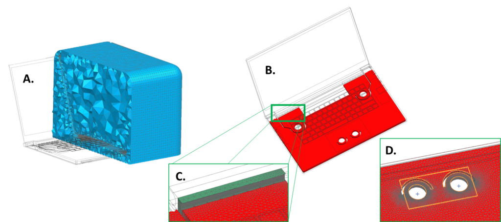
Figure 2 illustrates how a model is prepared for an acoustic analysis showing the finite element mesh of the air around the laptop (2A.), the interior mesh (2B), the connections between the interior and the exterior, the vents (2C) and the inlet grid under the laptop (2D). The next step in an acoustic analysis is defining the source region – this can be obtained from CFD or directly from -test data.
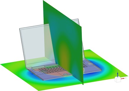
The equivalent acoustic source is calculated using Simcenter 3D and introduced into the FE model. Once solved, the sound field generated inside the laptop and that radiated away from it can be analyzed. Simcenter 3D enables the acoustic engineer to understand how the sound travels away from the laptop, the respective direction, and also reflections from the immediate environment.
Laptop OEMs need to understand the sound generated by the cooling architecture and investigate ways to minimize the impact on the user, like directing the noise away from the user via a rear-facing outlet. Additionally, the sound engineers can understand how the laptop screen shields some noise over a range of screen angles and user positions, as well as in the closed position if docked or connected to other monitors.
… and the sought-after “good” sound
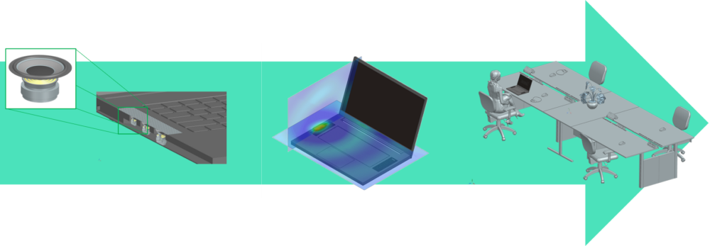
As mentioned in the introduction, sound quality from a laptop is regarded as an indicator of high brand quality. It is therefore pertinent for the engineer to understand the behavior of the speaker and how it performs within the laptop chassis. To optimize the sound and maximize the quality for the user, the engineer has to start with the standalone laptop loudspeaker and work through the subsequent integration into the laptop chassis up to the behavior of the laptop in a realistic user environment – see figure 3.
At the speaker level, as with all simulations, a geometry is defined from which the FE model is created and meshed. This structural vibration model of the speaker is then coupled to a small air volume near the speaker membrane. Specific acoustic radiation conditions are applied to the outer surface to permit predicting the far-field sound radiation characteristics. Simplified 1D models that are based on the Thiele-Small model are used as inputs for the coil loads. These models contain all the relevant electromagnetic-mechanical coupling effects in the speaker’s driver, and their input parameters are easily obtained from the supplier (or from simple measurements).
After solving the model, the sound radiation can be analyzed and post-processed to give directivity data, impulse responses, and distortion data. Figure 4 gives a graphical representation of this typical workflow.
Considering the speakers’ performance and association with perceived laptop quality, the engineer would be interested in quantifying the acoustic source strength and the uniformity of the sound field from the speaker. The image on the far right of figure 4 visualizes the radiated sound waves.
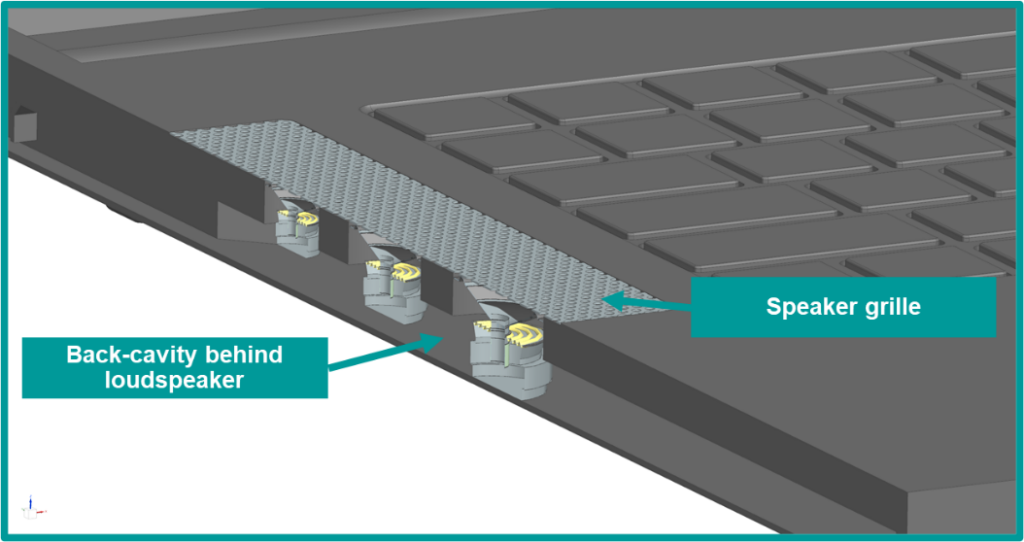
The next step is to understand how the integration of the speaker into the laptop affects the acoustic performance. In a laptop, the loudspeaker behavior is heavily influenced by the coupling of the speaker membrane with the air volume behind it and the visco-thermal effects that occur in the grilles that cover and protect the speakers from dirt and dust. The speaker model from figure 4 is therefore extended to also include the back of the speaker membrane to model the interaction with the back cavity within the laptop and the effect of the grille and the air volume between it and the speaker membrane as shown in figure5.
The effect of the grille can be explicitly simulated by:
- modeling the fluid in the holes and applying specific visco-thermal fluid properties or
- using simplified equivalent transfer admittance relationships.
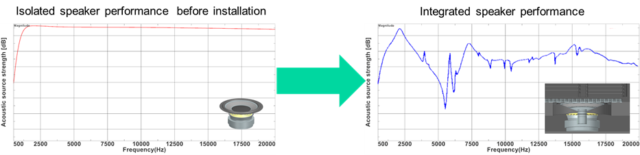
Figure 6 illustrates the effect the installation conditions can have on the speaker performance after integrating it into the laptop. For the isolated speaker, the left image in Figure 6, shows the speaker source strength to be uniform above one kilohertz. In comparison, the image on the right of Figure 6 illustrates a degradation of the performance above one kilohertz. There is very low sound radiation between the frequency range of four to six kilohertz and this is explained by the interaction between the speaker membrane and the resonance found in the back cavity. This is a more realistic evaluation of the speaker performance in the laptop and provides the design engineers with valuable insights to further optimize their product.
The final step in the process is to evaluate how the laptop will behave in its intended user environment – a typical office for example. However, to do so with a finite-element model would require significant calculation time and power. An alternative method is to use Ray Acoustics, one of the advanced acoustic solvers available within Simcenter 3D. This technology is based on ray tracing allowing it to effectively simulate sound propagation in wide spaces, over long distances and at high frequencies much faster than finite or boundary element methodologies ever could.
Model discretization and solution times are frequency-independent, making it perfect for solving problems where the geometry is larger than the acoustic wavelengths. Simcenter 3D offers both frequency- and time-domain results as an output from this solution. To simulate the office environment, three key modeling capabilities are available within Simcenter 3D:
- Edge and Surface diffraction – useful for typical partitioning walls within an office environment
- Curvature effect correction – accurate capture for discretized and meshed surfaces
- Absorption – both surface and air absorption
- Particle tracing – accounts for late reverberations and diffuse reflection effects typically encountered in indoor environments
The ray acoustic simulation model can directly compute sound quality parameters such as reverberation times, clarity values or sound transmissibility indices. Simcenter 3D can also directly incorporate the binaural effects in acoustic response without the need to model the human head – essentially obtaining the sound pressure levels that the left and right ears of the listener experience.
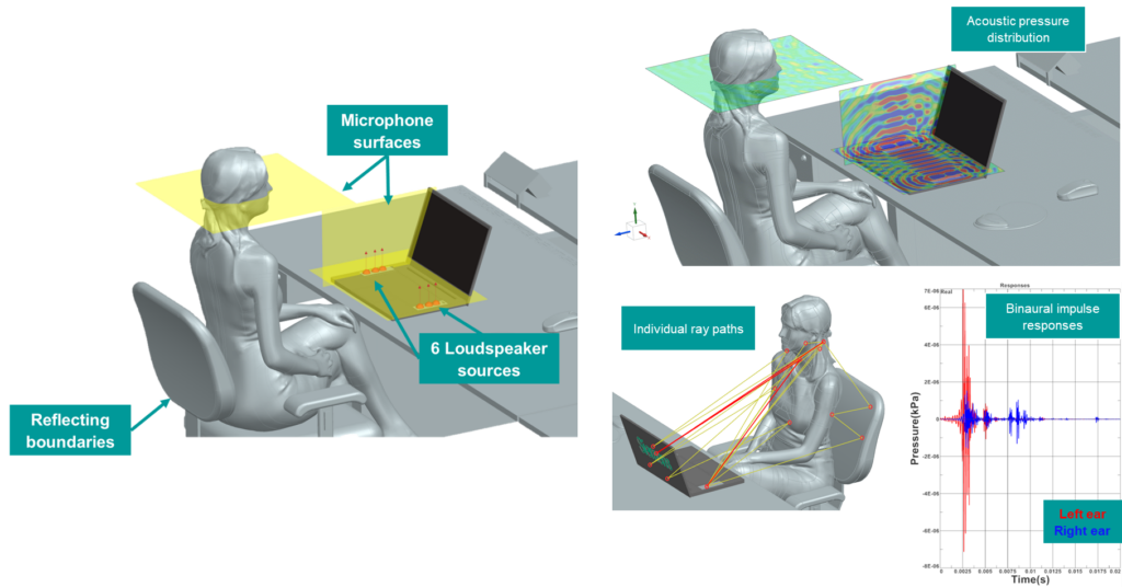
Figure 7(left) illustrates a typical office environment with all the reflecting or absorbing surfaces discretized using a simulation mesh (grey surfaces). Microphone surfaces near the laptop and the person’s head are defined to visualize the sound fields, as can be seen in the top right of Figure 7. Ray-tracing models offer insight into how the different combinations of speakers propagate to the person’s ear. Clear insight into how much sound is radiated to the user and how much is being reflected off the different surfaces can be unlocked using these ray-tracing visualizations.
Bringing it all together – a cacophony or a symphony?
All of the simulation steps discussed offer quantitative, visual information about the acoustic performance of the individual component through to product integration and the incorporation of it into the real-world environment. However, for all things sound, isn’t it best to be able to listen to the results of the simulations?
Simcenter 3D Acoustics offers a sound processing and auralization tool taking the results of the simulations and combining them with measured sounds like music to create acoustic scenarios that you can listen to!
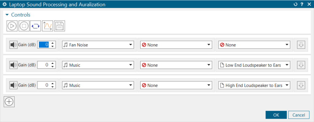
Figure 8 is an interactive image allowing you to test three different scenarios of a laptop:
- Noise from the fan simulation
- A piece of music that is played in the office environment using a low-end loudspeaker
- The same music played on a high-end speaker.
In the first scenario both the tonal and broadband components in the noise are present – auralization of it allows you to check how loud it sounds and how annoying or distracting it may be. In scenario two, how some music might mask the sound can be investigated –the noise of the fan is masked, but it is missing some low-frequency components of the music. Scenario three employs a high-end loudspeaker giving a much clearer and richer sound to the music.
Simcenter 3D Acoustics allows you to understand the sound and noise quality of your electric components. With these features you can design around the inherent noise and give the user of your products a more pleasurable aural experience.
Additional resource
Watch this webinar to understand how a combined simulation and test approach in the early design stages delivers critical acoustic performance insights and enables innovation in less time: Increase acoustic performance of consumer electronics using a combination of acoustic testing and acoustic simulation.