Speedy simulations: From Moore’s Law to more efficient algorithms

If your Computer Aided Engineering (CAE) resumé extends beyond 15 years in the field, you’ve seen a remarkable evolution in the speed and power of design and simulation software. The complexity of models that current software can now simulate is quite astonishing; consider this fully resolved turbulent simulation of a car in a wind tunnel.

Night and day is an accurate characterization of the difference between your early experiences as a CAD or CAE rookie vs. your current simulation capabilities. Two principle factors have contributed to the evolution of computer simulation performance. The first being the exponential increase in computer chip performance. The second, a continual improvement in predictive capability processing and algorithms on a similar scale.

Gordon Moore’s Optimism

“With unit cost falling as the number of components per circuit rises, by 1975 economics may dictate squeezing as many as 65,000 components on a single silicon chip.”

Gordon Moore

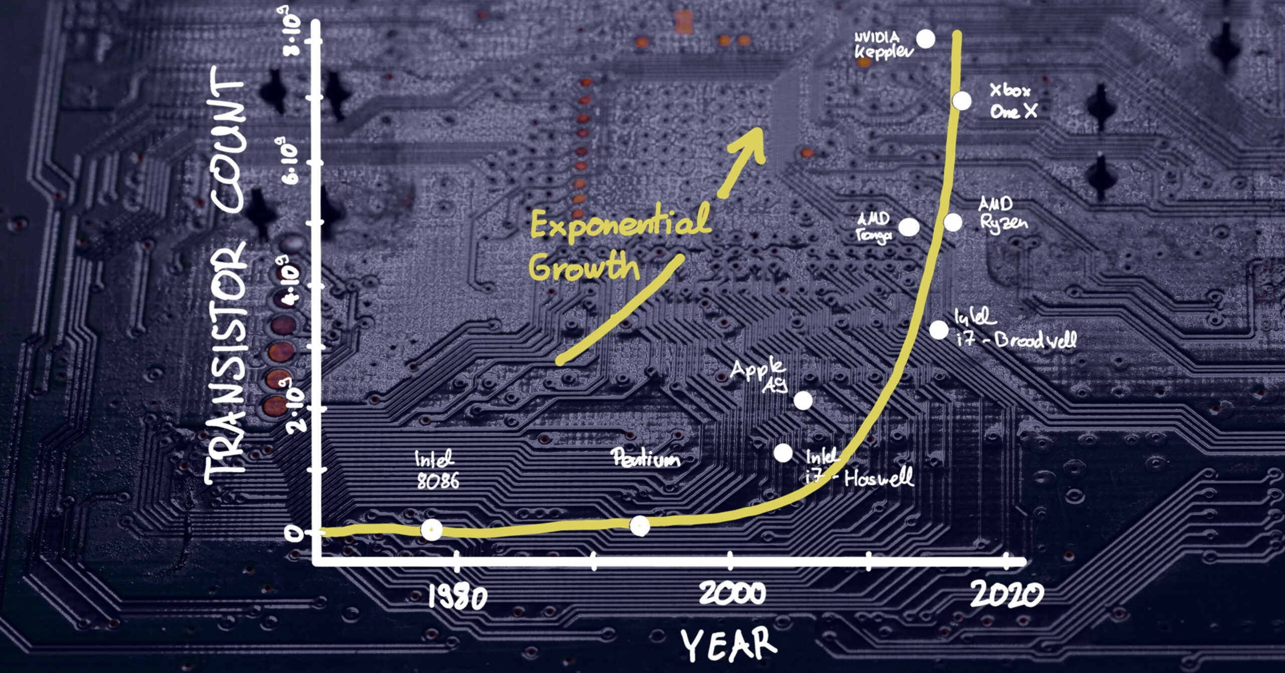
Intel co-founder Gordon Moore was nothing if not optimistic in April 1965 when he wrote these words as part of his seminal article, Cramming More Components Onto Integrated Circuits. Opining on the future of integrated circuits, he foresaw delivery of ever more powerful semiconductor chips at proportionally lower costs. What became known as Moore’s Law was his vision that the most basic Integrated Circuit would double in transistor density every year (a time window later expanded to 24 months) while remaining the same cost. The net effect would be the cost per transistor halving every two years. 

Moore’s Law became many things for the semiconductor industry; portentous enthusiasm, guiding principle and industry benchmark. As a target for planning and R&D, it certainly proved accurate with transistor counts now well into the billions. Consider that a modern smartphone has more processing power than NASA’s guidance computer used in the Apollo 11 mission during which Neil Armstrong took that famously giant step for mankind. Your average smartphone has 3-4 million times more rewritable memory than what was in the computers running the Apollo 11 lunar module and command module.

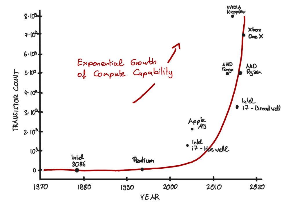
Moore’s Law itself is waning, however. In terms of its future relevance because it is starting to bump up against the physical reality (aka limits) of transistor size and semiconductor manufacturing capabilities. While some believe we’re already in a post-Moore period (Is Moore’s Law Really Dead?: WIRED), most experts remain optimistic that we will continue to see growth in computing technology. There is more-than-Moore, eg., highly parallelized architectures all the way to Quantum Computing.

Have you thanked an algorithm today?

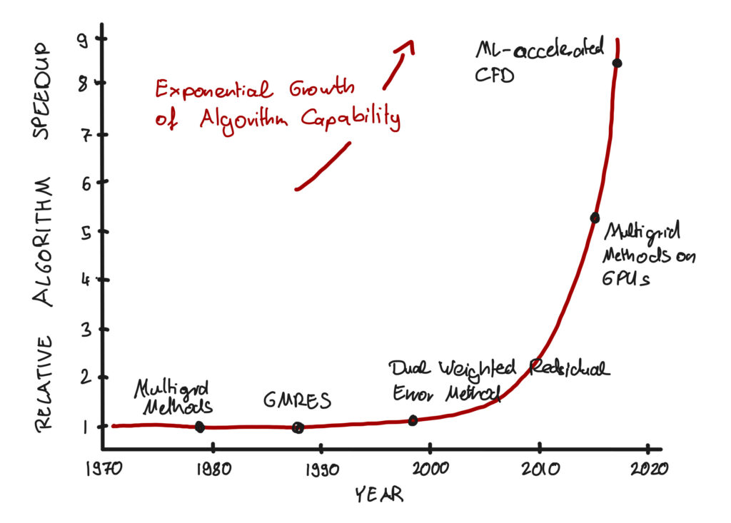
While Moore’s Law has been hugely consequential, the evolution in computer hardware alone would not have delivered the amazing simulation capabilities we now take almost for granted. A lesser-known contributor has been the improvement in algorithmic efficiency. Our ability to make algorithms faster and more capable is critical for simulation both in the present and the future. Let me share my enthusiasm and optimism from having both experienced and personally driven the exponential growth of algorithm performance during the last 15 years.

Algorithms in 2023 are far more efficient and rapid than before; a new algorithm running on a 20-year-old computer will generate a solution in significantly less time than a 20-year-old algorithm running on a new computer. Engineers can simulate more detailed geometries, intricate fluid dynamics, and complex physical interactions than ever. Complex simulations that once took days or weeks to complete can now be completed in hours or even minutes, allowing engineers to explore a broader design space and promptly make informed decisions. Furthermore, high-performance computing (HPC) systems can run simulations in parallel, significantly reducing simulation time as they test a much larger number of parameters and constraints.

Here are two areas, which underpin most simulation tools, where algorithms are improving:

1. Optimal discretization of physics equations

Let’s begin with discretization. 

The mathematical equations describing physics and driving simulations usually involve functions of continuous quantities such as velocity as a function of time and space. To compute these functions, they need to be discretized. Instead of using continuous fields, the computation is based on a finite number of variables in discrete locations in time and space (discretization points). This is done by reducing a continuous field such as velocity to many discrete quantities on a mesh or grid, where typically the vertices form the discretization points using discretization methods such as finite difference methods, finite volume methods, or finite element methods. 

Choosing an effective discretization method is crucial because it directly influences prediction accuracy and computation time. Increasing the number of discrete points and quantities increases the accuracy while also increasing computational time. In the past, choosing the best discretization method was a task best left to experts. Today, we have algorithms that provide us with valuable options:

• Opting for maximum predictive accuracy given a number of discretization points and using a mathematically optimal distribution of them
• Opting for a minimal number of discretization points – and thus optimal speed – yet still providing the requested accuracy for the given task

The corresponding algorithms are based on a very specific set of error estimations after each computation, which can localize the region where the highest error is occurring. In an optimization loop, additional discretization points are added to the areas with the most errors. This algorithmic evolution has meant that simulations run with an optimal number of variables to generate the desired accuracy level. Having an optimal number of variables is important since more variables require more computation time.

2. Linear Algebra – The major workhorse

Solving a system of linear equations is at the core of nearly every simulation tool. And in many cases, many hours are spent to solve them.

Solving a system of linear equations 101: Find a vector X such that A∙x=b, where X is of size n, A is a given matrix of size n∙n, and b is a given vector of size n.

Gauss elimination from the C18th (which you may recall from high school) is the most basic algorithm for this purpose, but computationally, it is extremely demanding. If you’ve forgotten high school, I’ll save you some Googling:

Gauss 101: If the number of variables is n, the Gauss algorithm is of complexity n³. That is, 10 times the number of variables will take 1000 times longer to compute.

In recent decades, mathematical researchers have continuously reduced the number of computations by exploiting the structure of the underlying systems. Today, we use multigrid methods to exploit the hierarchical structure of many systems. “Multigrid” means that these methods exploit spatial structure by solving the problem on a hierarchy of different computational grids. This is how we can solve systems of linear algebra with linear complexity. It’s exciting due to efficiency; when we increase the number of variables by a factor of 10, the corresponding system solution “only” takes 10 times longer instead of 1000 times longer using the Gauss algorithm. 

Example: Assume we’re solving a 3D physics problem and would like to reduce the discretization length by a factor of 2. That is, including twice as many discretization points in each spatial direction. This implies that we have in total 2∙2∙2 = 8 more grid points to solve for. Using Gauss’s algorithm, the computation would take 8∙8∙8 = 512 times longer. Using multigrid methods, however, it takes only 8 times longer or 64 times faster than the classic Gauss algorithm.

In the near future, the major workhorses of any 3D multi-physics simulations will be highly parallel multigrid algorithms specifically tuned for computer architectures such as Graphic Processing Units (GPU). This has already started and their powerful capabilities are already available in some simulation tools (as you can impressively observe in the video shown in the first section of the blog). Since we can no longer count on ever-increasing clock speeds, these type of massive parallel architectures will the key driver of computational power increases – one of the many More-than-Moore technologies. (The sharp increases in the stock market valuations of the leading GPU manufacturers indicate that this expectation is shared by many).

Moving forward

Moore’s Law is reaching its limitations and plateauing. That’s pretty clear. But what’s also clear is that computer technology will continue to improve due to new technologies in development or existing technologies getting better. For example, massively parallel computing architectures such as GPUs today and quantum computing tomorrow (figuratively speaking:)) will be hugely important. I’m super optimistic that we will continue to see exponential growth of computing power available to us.

Furthermore, I’m convinced that applied mathematics and computational algorithms will continue to be the foundation of innovation for the next 50-75 years. They have enabled us to realize innovations and products that many experts did not believe possible and will continue to do so. The combination of machine learning and classical simulation technology, for example, is creating completely new opportunities right now. I’m looking forward to discussing them and related topics in future posts.

---