Flexible spline curve control in the D-Cubed Dimensional Constraint Manager (DCM) – part 1
This article discusses techniques for creating and controlling flexible spline curves in the D-Cubed Dimensional Constraint Managers (2D DCM and 3D DCM). The examples given will focus on spline curves in the 2D DCM, but many of the principles can also be applied to splines in the 3D DCM. The article is aimed at anyone with an interest in developing curve sketching functionality in a CAD application environment. The article should be accessible to anyone with some previous background knowledge in the following areas:
- Experience of using a constraint manager, such as the DCM, and awareness of typical constraint types, such as coincident, tangent etc.
- Familiarity with the concept of constraint balance when adding constraints to a sketch (under-defined/over-defined geometry)
- Some awareness of basic NURBS concepts (spline degree, control points, parameterisation, interpolation conditions)
Objective
This article aims to answer some of the questions which may be encountered when a user-defined spline shape is incorporated into a geometric sketch. The main objective will be to create a curve which can maintain a characteristic shape whilst allowing additional constraints to be introduced between the curve and other sketch geometry. It is assumed that a constraint manager (the 2D DCM) is being used by the application to maintain geometric relationships in the sketch.
Interpolating splines lend themselves well to this task, by virtue of their properties:
- Natural curve shape
- Can achieve a close approximation to a given shape, by careful choice of the set of interpolation positions
- Can be constrained to other geometries, as part of a larger profile or can be a self-contained closed curve (for example, a periodic spline)
- Permit additional constraints and conditions to influence curve shape (direction at a given point on the curve, total length, tangent or coincident to other geometry)
Some situations which may be encountered when using interpolating splines include:
- Desire to minimise changes to spline shape, when adding constraints onto the spline. Generally, large changes to the shape will be less desirable than more local changes
- Inability to find a solution for a given set of constraints, due to adding too many constraints or conditions (over-defined geometry)
The approach taken in this article aims to address these aspects of spline solving behaviour, allowing close control of curve shape and robustness to changes in other geometry, without large changes in shape or over-defined situations.
Terminology – interpolating splines vs. control point splines
The article will make use of spline curves to generate a smooth curve shape which satisfies a given set of geometric conditions, such as a set of points which the curve must pass through. Spline curves lend themselves well to this task, enabling curve shapes to be derived to satisfy a given set of interpolation conditions.
In this context, we will make a distinction between interpolating splines, which allow a spline to be specified based on a set of interpolation conditions, and control point splines, which must be specified in terms of the control points that form part of the spline definition. Both interpolating splines and control point splines use the same underlying mathematical definition based on control points positions.
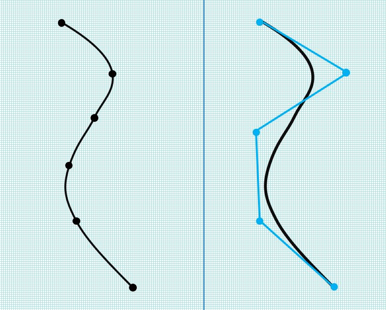
Figure 1: An interpolating spline and a control point spline
The DCM provides a dedicated spline curve type, allowing an application to specify an exact curve shape using a parametric NURBS-based definition. Constraints may then be added between the spline curve and other geometries. DCM provides two modes for adding spline curves, corresponding to the two classifications outlined above. In the current article, it will be convenient to work with interpolating splines, which delegate some of the spline implementation details to DCM and avoid the need to handle such details at the application level.
Controlling curve shape – approaches and limitations
Given a set of user-defined positions, we will aim to create a smooth spline curve which passes through the positions. It will be desired to connect the curve to other geometry in the sketch, using constraint types such as coincident and tangent. We will make use of the DCM’s interpolating spline functionality, specifying the user-defined positions as interpolation conditions for the spline. When adding an interpolating spline to the DCM, the application has the choice of creating a rigid, scalable or flexible spline curve.
As the name suggests, rigid splines maintain their initial shape, so the constraint manager may only transform the whole curve using rigid transformations (translations and rotations). This limits the edits that can be made to the sketch and no solution may be possible for particular dimension values or when adding new constraints.
Flexible interpolating splines are a DCM curve type which pass through a given set of positions but are not fixed in shape. This allows the DCM greater flexibility to satisfy user-defined constraints by modifying the shape of the curve. However, some application integrations may choose rigid curves to avoid sketch modifications forcing unwanted changes in curve shape.
Scalable splines allow the shape to be maintained, subject to one or two scaling freedoms (either isotropic or in two orthogonal directions). Discussion of these is beyond the scope of this article.
Table 1 summarises some advantages and disadvantages of the possible approaches:
| Spline type | Advantages | Disadvantages |
| Fixed or rigid splines | Guarantees no change in shape during constraint solving. | Cannot change shape to solve directional/tangent constraints onto other geometry. |
| Flexible spline with fixed interpolation positions | Allows the spline to remain flexible, subject to passing through the given interpolation positions. Overall spline shape is maintained. |
When applying additional constraints to a spline, it is may not be possible to find a solution as there may not be sufficient spline freedoms. |
| Flexible spline with interpolation positions added to DCM as free points | Possible to apply constraints onto the interpolation points, whilst leaving some freedoms. Less chance of over-defining the spline, due to the presence of freedoms in the interpolation points. |
Spline shape may change significantly when solving for constraints to other geometries. |
Table 1: A comparison of approaches for creating a spline curve based on user-defined points
A key differentiator between all these approaches is the availability of freedoms in the underlying spline definition. In the case of the rigid spline, each control point is relatively rigid to the other control points. This leaves the spline with no internal freedoms to reshape once the end point positions are fixed by constraints.
In the case of a flexible spline, the control points have positional freedoms relative to one another, but this does not necessarily prevent the spline from becoming over-defined. Each control point contributes 2 degrees of freedom to the internal freedoms of the spline, which are balanced by the freedoms removed by the interpolation positions. Fixing the interpolation positions will uniquely define the control point positions, leaving no freedoms to satisfy additional constraints (for example, a tangent constraint to another curve).
To define a spline passing through a set of interpolation positions which will support additional constraints, it is necessary to introduce additional freedoms into the spline’s underlying definition. Fundamentally, this involves the introduction of a new knot value into the spline’s knot vector, with a corresponding increase in the number of control points in the spline definition. The DCM spline interface allows an application to specify the knot vector for a DCM spline curve, but this requires an application to implement its own spline functionality, which the DCM spline implementation aims to make unnecessary. An alternative, more user-friendly approach, is to make use of spline interpolation conditions which will be explored in the remainder of this article.
Creating a flexible interpolating spline in DCM
Through spline interpolation conditions, the DCM provides another way for an application to increase the internal freedoms of a spline. When a spline with associated interpolation conditions is created, the DCM will generate a knot vector which provides an appropriate number of internal freedoms for the given interpolation conditions. Each interpolation condition must be assigned a ‘duration’ setting (see ‘Assigning durations’ below) which determines the permanence of the given condition when DCM modifies the spline shape in subsequent model evaluations.
Figure 2 below shows a degree 3 spline, together with 5 points which have been added as interpolation conditions. The position of each point defines an interpolation condition which the spline solution must satisfy. The positions of the underlying control points in the spline’s definition are shown, as the vertices of the blue control polygon.
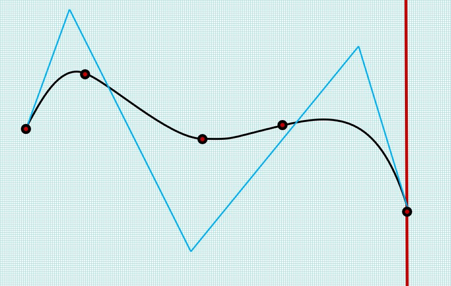
Figure 2: A degree 3 interpolating spline with 5 fixed interpolation positions
The number of control points is determined by the DCM and depends on the number and type of interpolation conditions being specified. In this case, 5 interpolation conditions (of type G_COI) requires a knot vector of length (interp_n + degree + 1)=8, which defines 5 underlying spline basis functions with 5 corresponding control points.
Crucially, the position of each point has been fixed in the DCM, removing the 2 positional freedoms from each point. By fixing the interpolation positions, all freedoms from the spline control points have been removed. The spline has no remaining freedoms and is well-defined – adding any additional constraints will over-define the spline*.
Increasing spline freedoms for end constraints
Suppose that the application needs to add a tangent constraint between the spline curve and the vertical fixed line. To avoid over-defining the spline curve, it will need to increase the internal freedoms of the spline, by adding a new interpolation condition. Since a tangency constrains the curve direction at the point of contact, a natural choice for the interpolation condition is the DCM’s first derivative condition type (DERIV1). Figure 3 below shows the spline curve after adding a new interpolation condition to the existing spline. In this model, a pair of first derivative direction (DERIV1_DIR) and first derivative magnitude (DERIV1_LEN) conditions have been added, which allows the direction and magnitude of the tangent vector to be controlled independently. The control polygon indicates that the number of control points has increased to 6, corresponding to the introduction by the DCM of a new knot value in the spline’s knot vector.
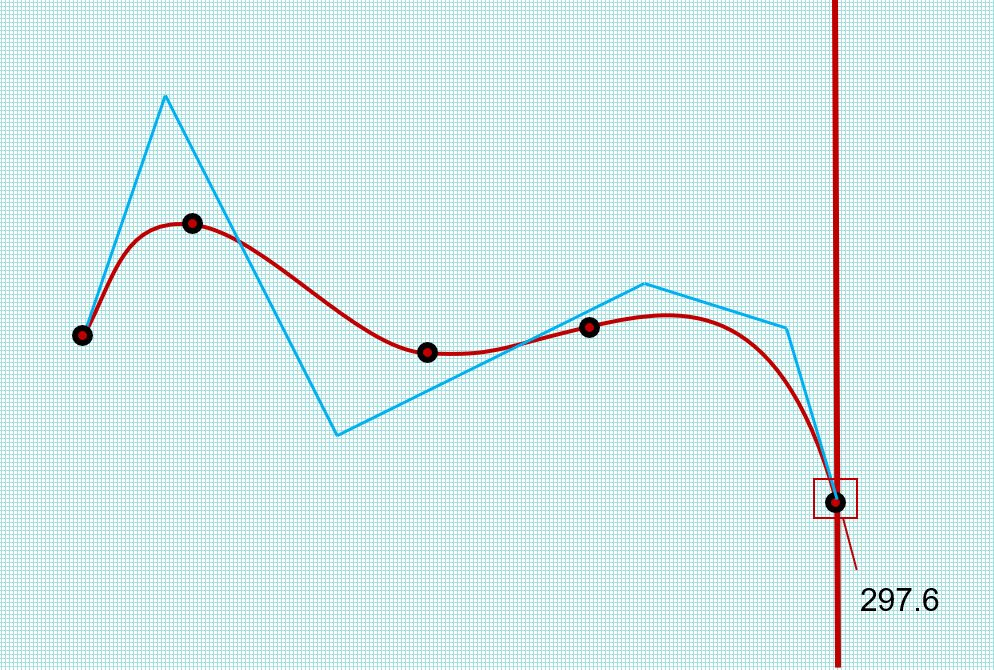
Figure 3: Increasing the number of control points in the spline’s definition by adding interpolation conditions
The new pair of interpolation conditions have been added based on the current tangent vector at the spline end. The spline now has sufficient internal freedoms to solve the given values of these conditions and remains well-defined. However, at this point, adding the tangent constraint between the spline and the vertical line will still over-define the spline, since the new derivative conditions have not been made available as freedoms to the DCM.
Assigning durations to interpolation conditions
DCM provides a ‘duration’ setting on all interpolation conditions – this setting can be used to release spline freedoms, allowing additional constraints to be applied to the spline. In the above spline configuration (Figure 3), the new interpolation conditions were assigned a duration of IDURATION_ALWAYS. This duration setting instructs the DCM to ensure the spline curve definition always satisfies the given condition, which has the effect of removing a freedom from the spline. Applying the tangent constraint will over-define the spline, since there are not enough freedoms in the spline definition**.
If the alternative duration setting of IDURATION_CREATION_ONLY is used, the DCM initially reports the model as under-defined, with 2 freedoms remaining. The conditions on the spline’s end tangent vector are used by the DCM to generate the initial spline shape, but the freedoms in the spline control points are still available during an evaluation. This allows additional constraints to be applied to the spline without over-defining it.
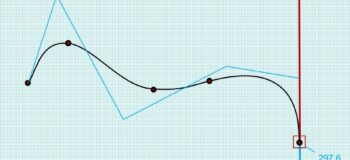
Figure 4 shows the same spline evaluated after adding a tangent constraint to the vertical fixed line, using the IDURATION_CREATION_ONLY duration for the DERIV1 conditions. The 2nd control point from the right is now positioned vertically above the right-hand side end of the spline, satisfying the tangent constraint. The direction of the DERIV1_DIR condition has also changed from its original direction shown in Figure 3 during the evaluation.
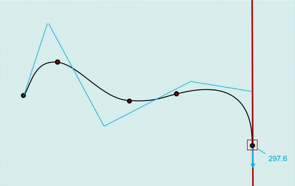
Figure 4: Modifying duration settings on interpolation conditions to allow a tangent constraint to be added onto the spline
At this stage, the spline remains under-defined and has one freedom remaining, since the tangent constraint removes only one of the two freedoms introduced when the interpolation conditions were added. Changing the duration of the DERIV1_LEN condition back to IDURATION_ALWAYS fixes the tangent magnitude and fully defines the spline.
This approach allows a spline definition to continue to pass through the specified interpolation conditions, but also provide enough freedoms to satisfy constraints to other geometries.
The example application code below demonstrates the creation of the spline in DCM, specifying interpolation points and derivative end conditions together with the tangent constraint to a fixed line.
In part two of this article, we’ll look at how DCM variables can be used to link the shape of a spline curve to control geometry, providing the end-user with further control of spline shape. We will also discuss choice of curve parameterisation and how it affects the shaping of flexible spline curves.
	// Example code showing the creation of a user-controllable interpolating spline
	// passing through a given set of interpolation positions.

	// The following code excerpt assumes that the calling application has
	// implemented and registered a set of DCM Frustum functions to provide
	// the necessary geometric data to the DCM
	// See the 2D DCM ex2 example program for an example Frustum implementation

	const int np = 5;				// Number of interpolating G_COI conditions defining the spline
	const int degree = 3;
	const int n_interps = np + 2;	// Total number of interpolation conditions (including DERIV1 end conditions)
	const double t_lower = 0;
	const double t_upper = 1;
	const double LIN_RES = 1e-8;
	const double ANG_RES = 1e-11;

	point*  anp[np];
	g_node* gnp[np];
	double g_coi_params[np];
	g_node* gninterps[n_interps];
	double params[n_interps];
	DCM_bs_itype itypes[n_interps];
	DCM_bs_iduration idurations[n_interps];
	double vectors[(n_interps) * 2];
	unsigned int interp_index = 0;

	dimension_system* dsp;
	dsp = new dimension_system(LIN_RES, LIN_RES / ANG_RES);

	// Create the defining points for the bounded spline
	// These will be added as g_nodes to DCM later on
	anp[0] = new point(-62.3, 31.8);
	anp[1] = new point(-44.4, 49.6);
	anp[2] = new point(-6.2, 28.7);
	anp[3] = new point(19.5, 32.9);
	anp[4] = new point(59.4, 5.2);
	g_coi_params[0] = t_lower;
	g_coi_params[1] = t_lower + 0.176*(t_upper - t_lower);
	g_coi_params[2] = t_lower + 0.4797*(t_upper - t_lower);
	g_coi_params[3] = t_lower + 0.6613*(t_upper - t_lower);
	g_coi_params[4] = t_upper;

	for(int ii = 0; ii<np; ii++)
		{
		gnp[ii] = dsp->add_g(anp[ii]);
		dsp->fix(gnp[ii]);
		}

	// Set the G_COI conditions
	for(int ii = 0; ii<np; ii++)
		{
		gninterps[interp_index] = gnp[ii];
		params[interp_index] = g_coi_params[ii];
		itypes[interp_index] = DCM_BS_ITYPE_G_COI;
		idurations[interp_index] = DCM_BS_IDURATION_ALWAYS;

		vectors[2 * interp_index] = -2;
		vectors[2 * interp_index + 1] = -2;
		interp_index++;
		}

	// Set the DERIV1 conditions on the right-hand end of the spline
	params[interp_index] = t_upper;
	itypes[interp_index] = DCM_BS_ITYPE_DERIV1_DIR;
	idurations[interp_index] = DCM_BS_IDURATION_CREATION_ONLY;
	vectors[2 * interp_index] = 10.3;
	vectors[2 * interp_index + 1] = -35.7;
	gninterps[interp_index] = NULL;
	interp_index++;

	params[interp_index] = t_upper;
	itypes[interp_index] = DCM_BS_ITYPE_DERIV1_LEN;
	idurations[interp_index] = DCM_BS_IDURATION_ALWAYS;
	vectors[2 * interp_index] = 297.6 / (t_upper - t_lower);
	vectors[2 * interp_index + 1] = 0.0;
	gninterps[interp_index] = NULL;
	interp_index++;

	// Create a fixed vertical line - later we will constrain this to be tangent to the right-hand end of the spline
	EX_vec_2d dir1(0, 1);
	line line1(anp[np - 1]->value(), dir1);
	g_node* gnLine1 = dsp->add_g(&line1);
	dsp->fix(gnLine1);

	// Make the spline
	spline sp(np, gnp);

	// Initial DCM_bs_data
	DCM_bs_data spdata;
	spdata.data_mask = DCM_BS_RIGIDITY | DCM_BS_PERIODICITY |
		DCM_BS_RATIONALITY | DCM_BS_DEPENDENCE |
		DCM_BS_PARAMETERISATION | DCM_BS_DEGREE |
		DCM_BS_INTERP_N | DCM_BS_INTERP_G_NODES |
		DCM_BS_INTERP_PARAMETERS | DCM_BS_INTERP_TYPES |
		DCM_BS_INTERP_VECTORS | DCM_BS_INTERP_DURATIONS;

	spdata.rigidity = DCM_BS_RIGIDITY_FLEXIBLE;
	spdata.periodicity = DCM_BS_PERIODICITY_NON_PER;
	spdata.rationality = DCM_BS_RATIONALITY_NON_RAT;
	spdata.dependence = DCM_BS_DEPENDENCE_INTERP;
	spdata.parameterisation = DCM_BS_PARAMETERISATION_CHORD_LENGTH;
	spdata.degree = degree;
	spdata.interp_n = n_interps;
	spdata.interp_g_nodes = (void**)gninterps;
	spdata.interp_parameters = params;
	spdata.interp_types = itypes;
	spdata.interp_vectors = vectors;
	spdata.interp_durations = idurations;

	DCM_bs_status spstat;
	g_node* gnSpline = dsp->add_spline_g(&sp, &spdata, &spstat);

	// Check return
	if(spstat == DCM_BS_STATUS_BAD_DATA)
		{
		cout << "Bad data: " << hex << spdata.bad_data_mask << endl;
		}

	// Constrain the fixed line to be tangent to the right-hand end of the spline
	dimension tan1(DCM_TANGENT);
	tan1.set_ends(&sp, &line1);
	tan1.set_help_parameter(&sp, t_upper);
	d_node* dnTan1 = dsp->add_d(&tan1, gnLine1, gnSpline);

	p_node* pnTan1 = dsp->parameter_node(&tan1, gnSpline, dnTan1);
	dsp->fix(pnTan1);

	// Evaluate the model to find a spline solution for the given constraints
	dsp->evaluate();

	dsp->erase(pnTan1);
	dsp->erase(dnTan1);
	dsp->erase(gnSpline);
	dsp->erase(gnLine1);

	for(int ii = 0; ii<np; ii++)
		{
		dsp->erase(gnp[ii]);
		delete anp[ii];
		}

	delete dsp;
*Excluding over-constrained but consistent constraint (OCC) schemes.
**Both DERIV1_DIR and DERIV1_LEN conditions each remove one internal freedom from the spline.

