Chaotic Fluid Dynamics Part 3 – Wheels

Rayleigh–Bénard convection involves the transport of heat from a hot bottom surface to a cold top surface. If the temperature difference between top and bottom is big enough, fluid rolls up into counter-rotating convection cells that transport the heat. Under certain conditions these convection cells flip-flop chaotically between rotating in a clockwise and counter-clockwise directions. Ed Lorenz’s famous ‘strange attractor’ is a graphical description of this behaviour:

A Pedagogic Example

The Malkus waterwheel is a fluid-mechanical model that intends to capture the same physical mechanisms as Rayleigh–Bénard convection. A tap/faucet supplies water at the top of the wheel, filling freely swinging cups positioned on the wheel periphery. Each cup has a hole in the bottom allow the liquid to slowly leak out:

As the cups are filled at the top, the wheel starts to move. If it moves too quickly, heavy cups rotating upwards tend the slow the wheel down. This results in cups being filled with more water at the top that then speeds the wheel up. The wheel flips between spinning in a clockwise and counter-clockwise direction. The red curve in the above animation is the center of gravity of the wheel, its path describes an attractor of the system.

As a pedagogic aid, the Malkus waterwheel is often used as an example of a chaotic system. From a thermo-fluids perspective, the added water is akin to ‘adding cold’ at the top, and the holes in the cups that let that water out can be viewed as ‘adding heat’.

A Thermosyphon Equivalent

So can CFD to be used to model a Malkus waterwheel? It’s quite a complex fluid-solid interaction application involving filling, sloshing and rotational dynamics, something that Simcenter STAR-CCM+ would be well suited to. However I’m going to take a slightly different approach, further abstract the application into an equivalent closed loop thermosyphon and use Simcenter FLOEFD for NX to simulate its behaviour:

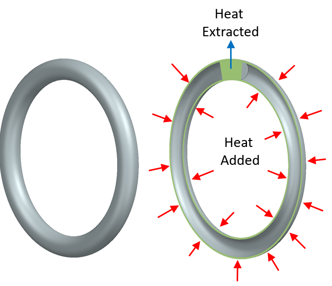
The loop is filled with water. Heat is extracted at a constant rate from a small volume of the fluid at the top of the loop (equivalent to water being added at the top of the Malkus waterwheel). Heat is added at a constant rate through the rest of the wheel (equivalent to the holes in the cups that let water out).

In which direction will the water flow? Let’s find out! (Spoiler alert – BOTH)

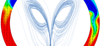
Water at the top is cooled down due to the heat extraction, water everywhere else heats up. The cold water drops down the inside of the tube until such time as it forces the flow in one direction, reinforced by the heated water pushing upwards on the other side. Round it spins until it slows down due to cold water being pushed up too far, the flow stalls, temperature drops quickly at the top (e.g. cup is filled with more water at the top when the wheel slows down), then it starts spinning again in a new direction. Sometimes the same direction, sometimes the opposite direction.

The flow is chaotic in that the number of spins in a given direction, and how often it changes rotation direction, are aperiodic:

Strangely Attractive

An attractor, plotted in so called ‘phase space’, is a way of collapsing a description of the behaviour of a system down into a bounded form. More useful than a time series plot that would go on for ever. It involves some integral properties of the system plotted against each other. Each point equating to a moment in time, joining the points up then shows a line that scribes a path.

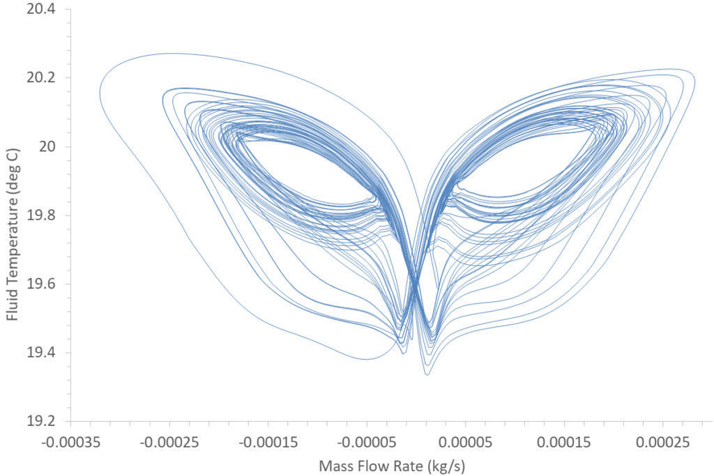
For this thermosyphon application, plotting the mass flow rate at the bottom of the pipe against the bulk average temperature at that plane creates a somewhat angry looking attractor:

Adding a 3rd property, the maximum temperature difference in the system at each time point, creates this 3D attractor:

If the system exhibited a fixed steady state behaviour its attractor would simply be a single point. Periodic time varying behaviour would be some kind of loop. An attractor of a chaotic system is called a ‘strange attractor’ in that the line never crosses itself, it keeps on going for ever. If it did intersect itself then it would have achieved an identical state to as it did previously and so go on to repeat that same (periodic) behaviour. A strange attractor is a fractal in that its dimension is fractional. A loop would have a dimension of 1. The Lorenz attractor has a dimension of 2.06, somewhere between a plane and a 3D solid and nope, I still haven’t got my head around that either.

Despite the fact that a meshed based CFD approach has been used to derive the above attractor, and it is of a system that is twice abstracted from classic Rayleigh–Bénard convection, it is heartening to see the similarity between it and the Lorenz attractor. Similar attractors can be observed in a number of differing fields, all going to show that there is a commonality to chaotic behaviour that underpins all physics (because there is only one physics, despite what you might have heard elsewhere).