Chaotic Fluid Dynamics Part 4 – Finding Feigenbaum
When forcing a non-linear dynamic system, be it a reproduction rate in a demography model or a temperature difference in Rayleigh–Bénard convection, a series of bifurcations are observed leading up to chaotic/turbulent behaviour. Mitchell Feigenbaum was the first to discover that the rate at which these bifurcations occur follow a universal pattern, irrespective of the type of non-linear system.
Feigenbaum’s Constant
In the mid 1970s Mitchell Feigenbaum was working at Los Alamos National Laboratories, tasked with applying renormalisation group methods to the study of fluid turbulence. Much like Ed Lorenz a few years earlier, he reduced the problem definition down to a time discrete iterated formulation.
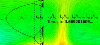
The logistics map was introduced in Part 1 of this series, showing how a system undergoes a series of period doubling bifurcations as it is forced from a constant state, through periodic behaviour then on into full blown aperiodic chaos. The rate at which these bifurcations occur can be quantified by looking at the relationship between the point of bifurcation and the forcing factor:
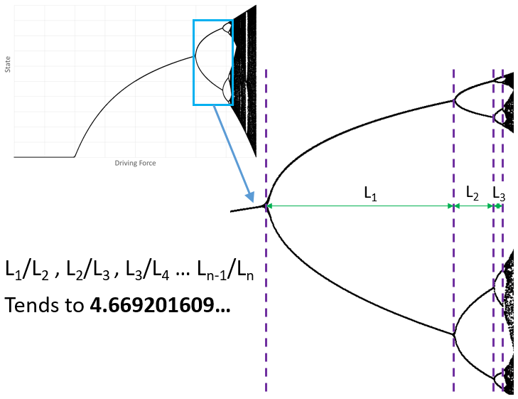
The genius of Feigenbaum was to both discover this constant value of 4.6692… and to recognise that it was the same regardless of the type of iterative function being considered. The only requirement was that the function had to have a single parabolic type maxima. The constant was not describable in any other way, e.g. it was not a function of any other mathematical constant. It was as fundamental as pi and e.
Confirmation from Fluids then Fame
His findings were rejected for publication a number of times until that is a publication by Albert Libchaber in Paris observed the same rate of period doubling behaviour in a Rayleigh–Bénard physical experiment:
Proof that Feigenbaum’s constant was not just a mathematical curiosity, but was observed in the ‘real’ world, propelled him to worldwide recognition and fame and by the mid 80s he was appearing on the front cover of popular magazines.

A Lifelong Desire
Although studying Mechanical Engineering at the time, I attended a free lecture in the Maths department of Brunel University in 1990 that introduced me to the logistics map and Feigenbaum’s constant. Fascinated, captivated and already beginning to focus on fluid dynamics and CFD, I included this ambition in my 1992 graduation yearbook, aged 21:

So, 30+ years later, let’s use Simcenter FLOEFD for NX to see if the constant can be observed through CFD simulation!
A 2D Rayleigh–Bénard model, air in a box with an aspect ratio of 2.4. Top cold wall is kept at 20degC, bottom hot wall heated in a (rather extensive) parametric study so as to identify the dTs that result in some change of the periodic temperature behaviour of a point in the middle, near the top of the box.
When dT reaches ~11.25 degC the flow begins to oscillate with a period of 1. The oscillations have just begun at this bifurcation point, so only a very slight ‘wobble’ can be seen in the 2D temperature + velocity streamline animation and the temperature variation at the probe point is very small:
The next point at which a change in the periodic nature of the flow occurs is at a dT ~22.625 degC. An extra frequency appears:
The dT only has to increase then to ~25.4 degC before the next change:
The final bifurcation point I could identify, prior to a bigger dT resulting in aperiodic behaviour, was at ~ 26 DegC:
These 4 dT bifurcation points allow the first 2 estimates of Feigenbaum’s constant to be calculated. First the difference between each transition dT:
L1 = 2nd point – 1st point = 22.625 – 11.25 = 11.375
L2 = 3rd point – 2nd point = 25.4 – 22.625 = 2.775
L3 = 4th point – 3rd point = 26 – 25.4 = 0.6
First estimate of Feigenbaum’s constant = 11.375 / 2.775 = 4.09
Second estimate of Feigenbaum’s constant = 2.775 / 0.6 = 4.63
All in all not bad compared to the theoretical limit value of 4.669201609… Lifelong ambition achieved!! 🙂
Simcenter FLOEFD as a Tool for Design Engineers
Admittedly these studies are a long way from the intended use of Simcenter FLOEFD, they are academic in nature and not examples of industrial product thermo-fluids design.
Simcenter FLOEFD is designed to be used primarily by mechanical design engineers who are comfortable working within an MCAD environment, may not have years of CFD experience but still have a requirement to investigate thermo-fluids behaviour of an intended product concept.
Unlike CFD power houses like Simcenter STAR-CCM+ with its broad range of application and depth of technology, all the numerics of Simcenter FLOEFD are preset; one turbulence model, one discretisation schems, a single Cartesian Octree based meshing approach. All tailored to enable repeatable predictions, with as little effort and pre-requisite experience as possible.
However, this does not mean that the predictions of Simcenter FLOEFD should be any less accurate or useful. And hopefully the above predictions go some way to demonstrate the integrity of Simcenter FLOEFD’s CFD technology.
For more standard industrial demonstrations of Simcenter FLOEFD, why not check out the following:
Extrusion tool design at Hager Group
Automotive air vent design at Dr. Schneider
[p.s. if you want to learn more about the life and works of Mitchell Feigenbaum (who sadly passed away in 2019), this article by Stephen Wolfram is a must read]
Chaotic Fluid Dynamics Blog Series:
Chaotic Fluid Dynamics Part 1 – Rabbits
Chaotic Fluid Dynamics Part 2 – Butterflies
Chaotic Fluid Dynamics Part 3 – Wheels
Chaotic Fluid Dynamics Part 4 – Finding Feigenbaum