Chaotic Fluid Dynamics Part 1 – Rabbits

“I am an old man now, and when I die and go to heaven there are two matters on which I hope for enlightenment. One is quantum electrodynamics, and the other is the turbulent motion of fluids. And about the former I am rather optimistic.” Sir Horace Lamb in an address to the British Association for the Advancement of Science in 1932

Turbulent fluid flow has both enthralled and frustrated scientists and mathematicians for centuries. For engineers turbulence can be both a benefit (e.g. mixing) and hindrance (e.g. aerodynamic drag). Although it might be argued we will never ‘fully understand’ turbulence, we have come some way in describing its behaviour.

So, with no further ado, let’s start with rabbits…

A Propensity for Procreation

Say we wanted to construct a mathematical model of a population of animals, some way of predicting how many animals there would be next year (Xn+1) based on the number this year (Xn). The simplest approach would be:

Xn+1 = r Xn

where r is the growth rate. If r = 2 then there would be twice as many animals next year as there are this year, twice the number the year after etc. Due to their propensity for procreation, rabbits are often used by way of example. Left unabated, the rabbit population would grow and grow. Not very realistic. The more rabbits there are, the less food resource each rabbit would have. Also foxes would have a field day. Let’s add a term to our population model that includes this predation:

Xn+1 = r Xn (1 – Xn)

Let’s also assume X, the rabbit population, is normalised to go from 0 (no rabbits) to 1 (max rabbits). The (1 – Xn) term gets smaller the more rabbits there are. Thus the more there are this year, the less they’d be next year, balanced with how well they reproduce.

A Fluffle of Rabbits

(Yes, a group of rabbits is called a fluffle, you couldn’t make it up. Though, as with all words, someone obviously did).

If the growth rate r is < 1 then the fluffle will eventually die out. If r > 1 then the fluffle population will evolve. Regardless of how many rabbits you start with, after a few years this is what the model predicts:

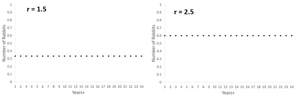
With these 2 values of r, the population reaches an equilibrium, the growth rate balances the predation. In fact the population will reach an equilibrium so long as r < 3. What happens if r > 3?

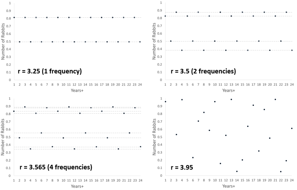
As r increases, the population first flips between 2 population levels in consecutive years, then 4, then 8. If r is big enough, the population becomes random (chaotic and unpredictable) year on year.

(Thank you for sticking with it and reading this far, don’t worry, there are some pretty cool animations further on)

The Logistics Map – Period Doubling Routes to Chaos

To see the entire scope of the behaviour of this model, we can collapse down the above graphs onto a single graph, showing the population X on the y-axis (?) and the value of r on the x-axis. For each value of r, iterate through the equation and plot a point on that column for values of Xn+1:

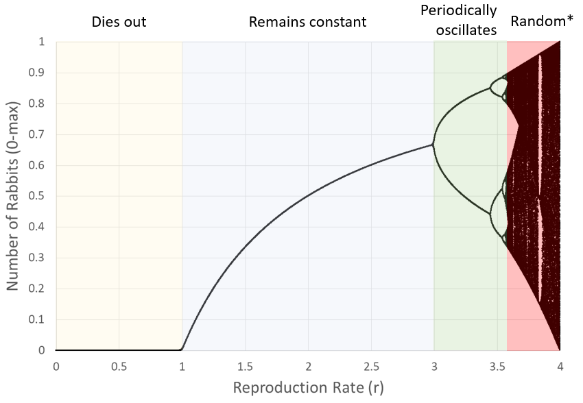
The graph is called the Logistics Map, popularised by Robert May in his 1976 publication ‘Simple mathematical models with very complicated dynamics’.

As r passes 3 the map bifurcates, a number of times, until r gets to 3.57 and the predictions become chaotic. Interesting to note though the windows of periodicity within the chaotic regime.

Although indeed derived from a very simple equation, the complexity of the logistics map has been observed in a range of fields. From the behaviour of lasers, atrial fibrillation, animal demography, the response of our eyes to strobing and (at last to bring this blog back on track) period doubling routes to fluid turbulence.

Rayleigh–Bénard Convection, with Wobbles

Take 2 horizontal parallel plates with a small gap between them. Fill with fluid. Heat the bottom plate. See what happens. Which is exactly what I did using Simcenter FLOEFD for NX! (technical details available on request if you want to replicate this model).

Depending on how big the temperature difference is between the bottom hot and cool(er) top plate, differing behaviours can be observed in the fluid flow and heat transfer mechanisms. Let’s start with a really small temperature difference, all the fluid between the plates starting at the same temperature as the top cold plate, and check out the transient response (blue-red colour represents the fluid temperature):

If the fluid gets hot enough, it will start to move due to buoyancy (natural convection). With such a small temperature rise, the fluid doesn’t move at all, it just sits there like a solid lump with the heat flowing through it due to conduction only.

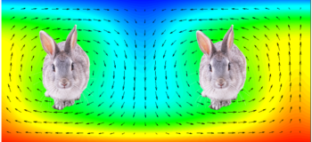
Now let’s increase the temperature of the bottom hot plate a little, show the evolution of the temperature (red through blue again), the flow vectors and a plot of fluid speed vs. time for a point in the fluid:

We have movement! After a while, the heat builds up enough to get the fluid moving. When it does, convection takes over and the flow rolls up into 2 counter rotating cells which do a great job of taking the heat from the bottom plate to the top cold one. The flow settles down to a steady pattern and stays in that state.

Right, let’s take it up another notch, increasing the hot plate temperature even further:

After it’s settled down, the flow (and temperature) then oscillates between 2 states (maybe you’ve figured out where I’m going with this).

Forcing the temperature up a little further still, we get another frequency appearing in the oscillations. A slight added ‘wobble’ that’s easier seen by plotting the speed (dark = slow, light = fast) instead of temperature. The point at which the velocity signal is measured is shown as a little dot just right of the middle, the animation shows the flow some time after the start:

Final one, let’s increase the hot bottom plate temperature even more:

Yep, you guessed it, the flow becomes chaotic, aperiodic, unpredictable, turbulent.

An Underlying Commonality

A person walks into a bar and asks the bartender “what’s the difference between period doubling routes to turbulence and fluffle demography?” The bartender replies “less than you might think”.

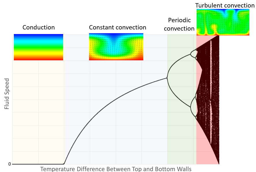
The logistics map and the Navier-Stokes equations are very different beasts. The commonality is that they are both non-linear and can exhibit various fractal properties (more on that subject in later Parts of this blog series). Although the above studies were not extensive enough to plot out an equivalent period doubling route to turbulence graph, period doubling has been noted in a number of experiments of Rayleigh–Bénard (and Taylor–Couette) flow. Taking a few assumed liberties, we can map the fluid behaviour to the corresponding sections of the logistics map

For this Rayleigh–Bénard flow, the point at which the fluid starts to move occurs at a critical Rayleigh number (~1708). ‘Back in the day’ I validated Simcenter Flotherm for this application, plotting Nusselt number vs. Rayleigh number to make sure Flotherm correctly predicted the transition from conduction to convection (Nu > 1):

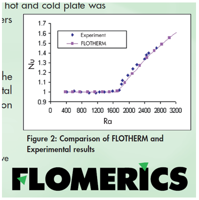
That graph looks suspiciously similar to the ~r=1 area on the logistics map, but maybe that’s the whole point!