The art of modelling using CFD. Part V – Grid
Any simulation technology based on an approach of subdividing a 3D model into many tessellated control volumes (e.g. the finite volume method) will be affected by the shape and size of those ‘mesh cells’ or ‘grid’. How fine should the mesh be to resolve the physics of the model being simulated? Good question. I used to ask my art teacher how to draw curtains. You don’t have to be a comic to figure out his answer to that one.
Grid provides the ability to resolve gradients of physical properties that your fancy say CFD tool is busy predicting for you. Gradients of temperature, air speed, pressure etc. If, in reality, a large part of your product has a pretty uniform temperature then from a modelling perspective you wouldn’t want to specify a lot of grid cells in that region. There’s no point, all the predicted temperatures in those cells will be the same, might as well use just one or two cells. Cells make the solver take memory and time to reach a prediction. Too many cells = unnecessarily slow solution.

Take the smiley above. How many cells (pixels in this case) do you need to recognise what the image actually is? Less than the following apple tump:
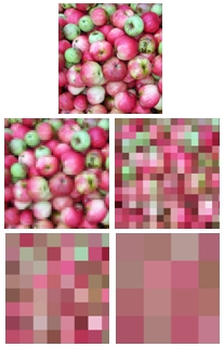
The apple tump is more ‘complex’, there are many more gradients. Let’s go from pixels and recognition to grid cells and simulation accuracy. I’ve used FloTHERM to do what is called a grid sensitivity test on a real simple example, a pcb with 3 powered components sitting in an air stream. Starting with a real course grid, in fact a minimum structured grid required to resolve the geometry, what us FloTHERMians call a ‘keypoint grid’. I then increased the grid density everywhere in the model 4 times and plotted the resulting temperature predictions:
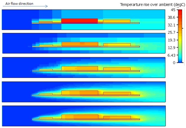
You can make out the mesh size by looking at the colour variations, each grid cell has a single temperature prediction / single colour in it, that’s as much as the solver can do (from a finite volume perspective). After a while the results don’t change much, they become ‘grid independent’. This graph shows the component temperature predictions at all the various grid sizes spanning the above 5 models:
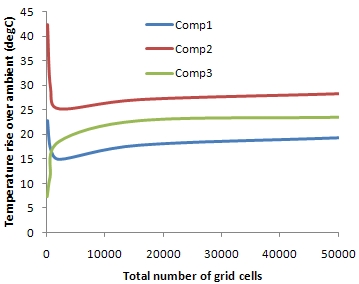
Not an atypical plot. Comp3 (the one most downstream) has a different trend than the other two, it’s final temperature is much more dependent on the effect the other upstream components have on the air flow. The 50,000 cells of the finest level are distributed equally everywhere. The real art of gridding is to know where in a model a fine grid is required and where you can get away with a course grid. Visual inspection of even a medium grid density result will enable you to figure out where to cluster your cells. Experience tells us that you need fine cells at all solid/fluid interfaces where there is a critical amount of heat transfer from (e.g. top of all active components, top and bottom surface of the PCB). If you haven’t got the time to gain such an experience then no worries, we’ve automated gridding of PCBs in both FloTHERM PCB and FloEDA Bridge (FloTHERM’s EDA interfacing application window). Such standard geometries lend themselves readily to automated gridding rules that balance grid independence with total grid number minimisation. For the above application our automatic gridding rules enable a solution that is <5% from the grid independent solution with only 6 thousand cells. If your electronics thermal CFD tool doesn’t have such automatic gridding rules then check FloTHERM and FloTHERM PCB out.
4th June 2010, Ross-on-Wye