The beauty of optimization: what ears and mufflers have in common
Beethoven’s life was marked by the tragedy of his deafness, for which symptoms appeared in his latest twenties. Before being completely deaf, he used ear-horns to improve his hearing condition, tools that visitors can see at the Beethoven’s museum in his native Bonn [1]. Unfortunately, his problem had most likely a severe pathological origin and such tools did not help him significantly throughout the years [2]. The first record of ear-horns usage dates back to 1634 when the French Jesuit Jean Leurechon describes them in his writings. Their main scope is to convey acoustic waves towards the ear but they disappeared around the 60thies in favour of more practical medical devices.
Now, if you are familiar with natural evolution, you are maybe wondering why we did not end up having cone-shaped ears to enhance our hearing capabilities? At the end of the day, the ear function is to make us hear. The problem is that ear-horns work well only if the person points them towards the sound source: a cone-shaped ear would have prevented us to individuate the provenance of sounds, quite dangerous even for our survival. Another aspect tied to the human ears, is their ability to better capture sounds at frequencies typical of the human voice. Basically, we have human ears to listen to the human voice. All in all, natural evolution had to optimize the ear topology, a process that took millions of years, to satisfy several criteria and objectives without compromising any aspect.
Speaking of which, what is sound? Sound as we know it, becomes fascinating because of the way our human brain processes it. In reality, sound is much more banal and it is nothing but a mechanical vibration propagating in a medium, obeying to all the laws of nature related to waves. Sound is thus subjected to reflection, refraction and diffraction. Such capricious phenomena are of course a nightmare when dealing with engineering design. The first example that comes to my mind are the acoustic waves produced by the heat-release fluctuations in a gas turbine flame. These waves can travel in a combustion chamber and perturb the flame. Even worse, they can amplify and make combustion unstable. If you are a gas turbine engineer, you have all my sympathy.
If you are a muffler engineer, your life won’t be easy either. The muffler is a device at the very end of the powertrain, which suppresses the acoustic waves coming from the engine. The acoustic loss is triggered by abruptly changing the area of internal ducts (expansion chambers), creating reflected waves that can cancel out the incoming waves, or by absorbing the acoustic energy, for example by means perforations in the ducts that connect with a volume filled with a porous material. As usual in engineering, “you never get something for nothing”. There are two pieces of bad news in this scenario: the first is that the muffler presence increases the backpressure, thus decreasing the overall efficiency of the engine. The second bad news is that increasing transmission loss and decreasing backpressure in a muffler are concurrent objectives. I told you: muffler engineer life is not easy. But in this blog, we’ll try to crack the code anyway.
 Figure 1: the optimization workflow
Optimizing the muffler design during manufacturing is quite cumbersome. In a normal manufacturing processing, engineers do not optimize backpressure and noise reduction at the same time. In the current industrial processes, backpressure is reduced through geometry optimization; noise reduction targets are verified only in a second phase and the whole process strongly relies on the engineer’s experience. It is time consuming and engineers can build and test only a few designs. That is why a combined approach is more convenient and highly desirable. In this blog we will introduce you to a new approach combining HEEDS (Simcenter optimization tool), Simcenter 3D to deal with the acoustic part, and Simcenter STAR-CCM+ to provide the backpressure prediction. Figure 1 provides the example of the workflow. The optimization is performed in HEEDS with the algorithm SHERPA, which selects a set of geometrical parameters at the beginning of the iteration. Such set is read by the CAD modeller NX, which builds a parasolid model that can be read by both Simcenter STAR-CCM+ and Simcenter 3D. Simcenter 3D calculates the transmission loss, defined as the ratio between the acoustic power at the inlet and the one at the outlet, as a function of the inlet noise frequency. Of course, SHERPA will try to maximize the transmission loss, as higher values translate into a larger noise reduction. At each iteration, a coefficient CF is calculated to measure the distance between the transmission loss-frequency curve from the baseline one. When both Simcenter STAR-CCM+ and Simcenter 3D provide the calculation response, SHERPA decides on the new set of parameters that can satisfy the objective.

Figure 2: Pareto front of the optimization study.
I admit, as CFD engineers we might get a little snobbish when looking at the only apparent unstrictness of economy laws. Yet, to crack the code, we will use a concept directly from the Italian economist Vilfredo Pareto. Apart from the 80/20 rule, he also gave life to the Pareto front, useful to individuate the concurrency between the objectives. Figure 2 shows the Pareto front for this study, function of the backpressure and CF, with the light blue area showing unfeasible designs. It is possible to distinguish three different regions. Region 1 shows a clear Pareto front tendency when two objectives are concurrent: in this case the higher the transmission loss, the higher the backpressure. Region 2 is a region of low backpressure whilst Region 3 is a not much populated region. It means that SHERPA focused solely on Region 1 and 2.
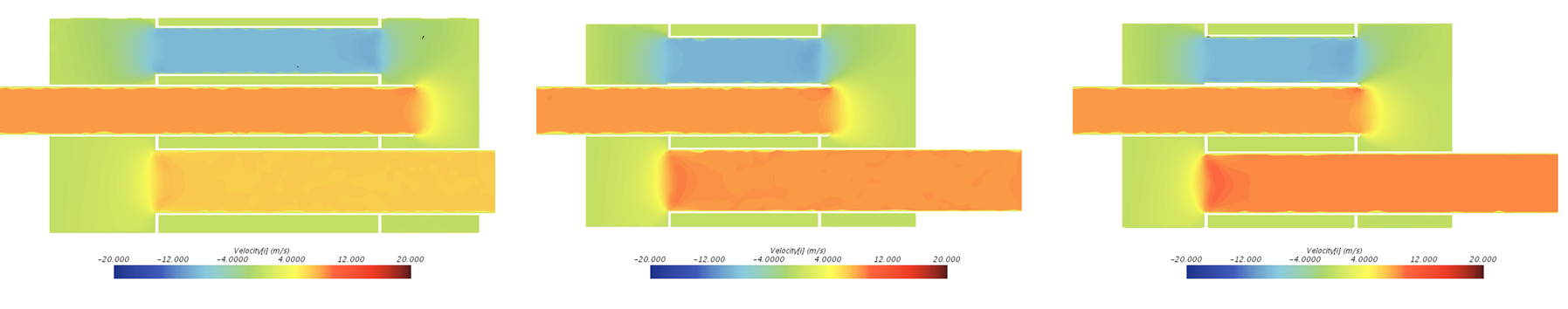
 Figure 3a (left): Baseline; Figure 3b (center): from Region 2; Figure 3c (right): from Region 1;
 Figure 3da (left) and 3db: both from Region 3;
Little golden rule: SHERPA is a fantastic algorithm, but the critical analysis of the results from the human engineer is still necessary. Figure 3 and its subfigures aim to understand the results. Figure 3a shows the baseline design, in which you can notice distinct three chambers in which the flow is forced to pass through. Figure 3b is representative of Region 2, a region with low backpressure. As you can see, the internal chambers collapsed together, with the gas flowing directly from the inlet to the outlet. Although for SHERPA this is a feasible design, in reality this is not a real muffler configuration. This can suggest that we have a physical limit in decreasing further the backpressure of our baseline. Therefore, Region 2 is discarded. Figure 3c comes from Region 1. In this region all the designs are valid designs, with the typical three chambers structure for a muffler. As said above, in this region we are not able to increase the transmission loss and decrease the backpressure at the same time. Figures 3d are more interesting: they come from Region 2 in which we can observe both valid (Figure 3da) and non-valid (Figure 3db) designs. More interestingly, this region is placed in backpressure values below the baseline design, with a good potential for improvement. However, Region 2 is scarcely populated and yet, it’s exactly there that our best designs will be found.
 Figure 4: Pareto front of the detailed study. Boundaries for backpressure are set within 4100 and 3200 Pa.

Figure 5a (left): Baseline; Figure 5b (center): Backpressure reduced by 9.7%. CF=1.09; Figure 5c (right): Backpressure reduced by 6.8%. CF=1.70.
SHERPA allows you to be a perfectionist. The improved design of Figure 3da is only the starting point of our analysis. We start to see the light at the end of the tunnel, but in my opinion, we did not crack the code yet. From the first optimization study, we observe that at very low backpressure we do not obtain valid designs. For this reason, we are now asking to SHERPA to build designs in a region in which backpressure has a lower and upper limit. The resulting Pareto front is represented in Figure 4. The designs in the red area are all valid designs, with both an improvement in backpressure and the coefficient CF, actually a very good news for our target. Ready to elect the best design?! We actually have two good candidates, highlighted in Figure 4 as A and B. They present very similar geometries. Depending on the final design requirements, the engineer will decide whether to manufacture design A (with an improvement of 9.7% of the backpressure) or design B (with an improvement of 6.8% of the backpressure, but with a higher CF). Designs A and B are reported in Figure 5, along with the baseline. As you can notice, the geometries are quite similar: in other words, the variations obtained on the final targets, are actually the result of very tiny geometrical variations. This can also be observed with one my favourite HEEDS tools: the parallel plot (Figure 6). This plot allows you to individuate designs that provide the desired responses and to see the boundaries within which their geometrical parameters vary. In the x-axis, we plotted the backpressure, the coefficient CF and the geometrical quotas varied by SHERPA during the studies. We highlighted in blue only the designs falling in the valid Pareto front of Figure 4. These designs bundle together and their geometrical quotas are varying in a very restrained interval, suggesting that all these designs are indeed quite similar. Yet, they have a strong impact in the final response.

Figure 6: Parallel plot for the detailed analysis. a* are geometrical variables that were modified during the studies. Results are filtered for backpressure (3200 Pa <backpressure< 4100 Pa) and CF (0 <CF< 5).
I finish the blog with one open question: our hearing capabilities took more than hundred millions of years to evolve. Do you think that SHERPA would have reduced the time to optimize the ear topology? I am firmly convinced that the answer is yes!
References
[1] Beethoven’s ear-horns in Bonn