STAR-CCM+ v11.06: Building a better sim file – part 1 of 2

Please note: Original publication date 10-18-2016
A well organized workshop, purposely conceived to build and revise things of interest, is truly appealing with its array of tools, carefully ordered, in a familiar and comfortable environment. Now you’ve probably heard the expression “Use the right tool for the right job.” That works when you know what tools you have in your workshop, what they are supposed to do and exactly where you can find them. With the STAR-CCM+® v11.06 release, we’re adding and upgrading tools that will improve your ability to productively build and revise your simulations. You’ll be able to set up your simulations more comprehensively and consistently with a reduced likelihood of errors. And you’ll be able to more efficiently conduct critical reviews in the deeper details of your simulations with your colleagues and your customers. In part one of this blog, I’ll be talking about Simulation Parameters and Global Tagging.
Before STAR-CCM+ v11.06, when you wanted to specify a constant for use in multiple locations, or as a part a more complex expression, you created a field function – a simple scalar, vector or tensor. But there’s an overhead – a field function is evaluated and stored at every cell. That can become expensive when all you need to store is a single constant. This is perhaps the key difference between simulation parameters and field functions – the former objects, being “spatially invariant,” only need to be stored once. Here are a few other things you need to know about simulation parameters: they can be defined as either scalars or vectors; referenced by other simulation parameters; be used in field functions. You can use them in our 3D-CAD tool to modify geometry, or anywhere that you can use either a field function or type-in expression now. Let’s consider a biomedical application, where we have a notional drug delivery catheter in place near a stenosis in an artery (shown below).
 A tracer released at the catheter inlet and exiting from the holes in the catheter is shown using volume rendering. The artery inlet flow speed (left axis) versus time is shown in the plot (lower right). Expression reports which calculate the bulk tracer concentration are set up for six planes (A thru F) along the axis of the artery and are also plotted versus time (right axis). Per-part reporting (also introduced with STAR-CCM+ v11.06) simplifies the creation of the expression reports used in this quantitative assessment of drug delivery.
At the upstream inlet, the annular space between the artery wall and the catheter outer wall, we can use an analytical equation [1] to apply a fully developed flow profile. We define simulation parameters (Xs) for the artery wall radius, the outer catheter wall radius and the mean flow rate and use them in a field function (fxs) for the steady velocity profile. Now, the arterial flow rate also changes in response to the cardiac rhythm. Again, there is an analytical equation available [2] that takes this into account. We define simulation parameters for the pulse rate, BPM (beats per minute), and the value of PI . A second time varying field function (fxs) for the unsteady velocity profile incorporates the steady velocity profile and these additional simulation parameters (Xs). Taking this one more step, we’re going to consistently set the time step for our Implicit Unsteady solver by encapsulating our BPM simulation parameter within another simulation parameter – when we change the flow rate, as defined by BPM, the time step can be automatically changed.
 Use a simulation parameter BPM to set the time-step size used by the solver.
We’ve now built a simulation ready to study a range of flow rates in the most physiologically realistic way that also lets us explore a broad combination of patient physiologies and catheter sizes. It’s handy to be able to get an overview as you work on a simulation effort. That starts with good organization, and this is where tagging comes into our discussion. Tags aren’t new; they’ve been around for a while. But they’ve gotten a major upgrade in this release – they are now available for nearly every object on the simulation tree. Tags give you a way to connect objects that might not otherwise be easily or logically associated. Let’s go back to our biomedical application. First, we’ve created tags called “problem_setup” and “instrumentation” with the intent of identifying objects on the tree that are associated with either the setup of the problem, or are needed for quantitative and qualitative assessments of the results. Some objects are associated with both, and multiple tags are allowed. This exercise is something that can be ideally done while you are building your sim file.

Next, we create a Custom Tree (one of our top features in STAR-CCM+ v11.04) directly for each tag. This makes it easier to see the connection between our simulation parameters, field functions, and where they are actually used. We can easily check that our simulation is properly instrumented before we start our transient run. These tag-based custom trees let us efficiently review our simulation with other colleagues to potentially catch any errors or omissions. In the end. We expect that being able to efficiently scrutinize a problem setup before submitting it will increase the confidence in our analysis setup and any conclusions that we’re able to draw from the results.
In the animation above, a tracer species, released at the catheter inlet and exiting from the holes in the catheter is shown using volume rendering. The artery inlet flow speed (left axis) versus time is shown in the plot (lower right). Expression reports which calculate the bulk tracer concentration are set up for six planes (A thru F) along the axis of the artery and are also plotted versus time (right axis). Per-part reporting (also introduced with STAR-CCM+ v11.06) simplifies the creation of the expression reports used in this quantitative assessment of drug delivery.
We started our discussion by recognizing that you need the right tool for the right job. That’s certainly true, and it’s also fair to say that you’re only as good as your tools. We hope that simulation parameters and tagging will truly help you to build better sim files that are easier to understand, run more robustly, and in the end, repeatedly deliver highly accurate results that you can be confident in.
References
[1] Bird RB, Stewart WE & Lightfoot EN, Transport Phenomena, 3rd printing, John Wiley & Sons; 1960.
[2] Womersley JR., Method for the calculation of velocity, rate of flow and viscous drag in arteries when the pressure gradient is known. J. Physiol. 1955; 127:553-563.

Comments
Comments are closed.