Breaking the Courant Number barrier for multiphase flow
Multiphase CFD simulation and Courant Number
Aliens had just crashed in New Mexico (allegedly), India and Pakistan had just gained independence from Britain, and Hillary Clinton was just about to be born. The year was 1947, two years after the end of the war, and a long-standing barrier was about to be broken… I refer of course to the so-called sound barrier, so called because in the end it turned out to be no barrier at all.
In the years that led up to that celebrated moment, it had been believed by many that it was impossible to break the sound barrier in a controlled way. Many had tried and failed. On each occasion pilots encountered great instability and came close to losing, or even lost control of their aircraft. Compressible flows were not well understood at the time and shock waves formed on wings and control surfaces. These altered the aerodynamics so much that aircraft struggled to stay airborne, particularly as control surfaces were mechanically operated and pilots were no longer able to move them.
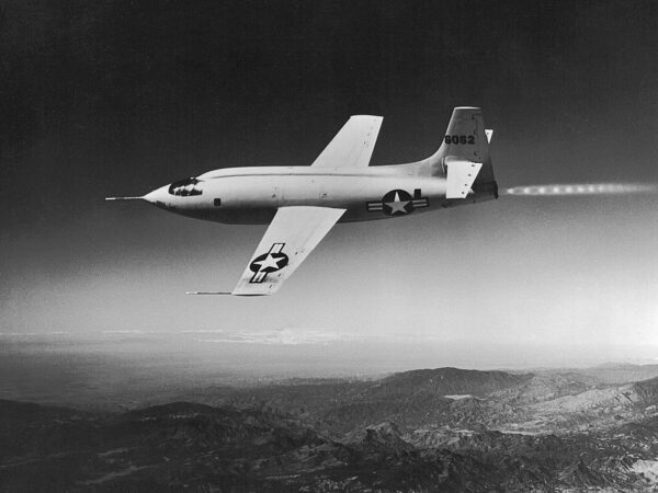
All of that was to change on 14th October 1947, when after years of research by the British and the Americans, Chuck Yeager was the first pilot to officially (and controllably) break the sound barrier in the Bell X-1. The barrier had been overcome by doing things differently. The Bell X-1 was designed with control surfaces that were now actuated instead of being manually operated, and the whole surface moved as a single part to avoid the large moments previously experienced on the fixed-flap arrangement.
As CFD engineers working with multiphase flow applications, we face a similar barrier – the Courant Number barrier! If we want to simulate applications with free surfaces using the Volume Of Fluid (VOF) method, we cannot exceed a Courant (CFL) number of 1 without significantly compromising the accuracy of our solution and the value of the results. This is because VOF is designed to do one thing – to capture sharp free surfaces between immiscible fluids. To do this, it is important that the free surface does not move across more than one cell in a timestep, otherwise the solver will smear the interface over multiple cells giving rise to the dreaded numerical mixture. Whilst this mixture may look like a real mixture, and in some cases, mirror a physical mixture, there is no modeling of the interaction between phases. As a result, once a numerical mixture exists it will not separate into distinct phases again and will continue to pollute your results, particularly in closed domains.
This October’s release of Simcenter STAR-CCM+ 2020.3 is about to change all that; the long-standing Courant Number barrier is about to fall… Enter MMP-LSI!
One Model to Rule Them All
The MMP in MMP-LSI stands for Mixture MultiPhase, one of our existing multiphase flow models in Simcenter STAR-CCM+ that is suited to modeling (as the name suggests) mixtures. This model is from the same root as VOF, it is single phase plus a volume fraction. In fact, if you remove the HRIC interface sharpening from VOF and add a slip model to account for the difference in velocities between phases you more or less have MMP.
This commonality is something we can make use of if we want to come up with a model that can both capture free surfaces and model mixtures. That model is MMP-LSI.
LSI stands for the Large Scale Interface model, and some of you may recognize this as a model we have previously released for Eulerian Multiphase (EMP), but now under MMP, we have a model that is much more lightweight, and that can produce similar results to VOF in areas where the CFL number is low enough, but can still model mixtures that can separate under body forces such as gravity or centrifugal loads, something VOF cannot do. Moreover, if we have a limited budget (who doesn’t), we can choose to resolve the larger structures with free surfaces but allow smaller structures such as droplets or bubbles to be modeled as a mixture. Resolve what you can, model what you can’t in an approach similar to hybrid turbulence modeling. This is multiphase flow modeling redefined.
What does this mean to me?
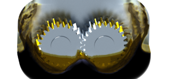
The best way to understand how MMP-LSI can help us as engineers is look at an application, in this case gear lubrication. Typically, the problem with such applications is that the gears rotate very fast and generate a large number of very small but fast-moving droplets. This presents a challenge for VOF as resolving these small droplets and the associated timescales make for a very expensive simulation. A typical thing that engineers try to make such simulations tractable is to increase the time-step size, but with VOF this just leads us to a numerical mixture and often unusable results. With MMP-LSI, however, we can do exactly this and still get good results.
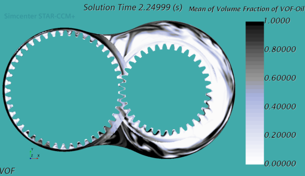
In the example below, two intermeshing gears in an oil bath are modeled with overset using first VOF and then MMP-LSI. Adaptive time-stepping is used to control the timestep so that the maximum CFL number can be controlled in the region of free surfaces. This allows us to set a value below 1 if we intend to resolve the free surfaces, but with MMP-LSI we can set a higher CFL number.
Adaptive Timestep
CFL=0.5
VOF
Ave. Timestep = 8.52e-5s
MMP-LSI
Ave. Timestep = 6.88e-5s
CFL=5
Ave. Timestep = 9.22e-4s
Ave. Timestep = 5.12e-4s
Let’s look first at the resolved cases where a CFL number of 0.5 was used. Both VOF and the MMP-LSI runs show well resolved structures throughout and produce very similar flow patterns. MMP-LSI can be seen here as a substitute for VOF. The adaptive time-stepping produced a smaller timestep for the MMP-LSI case but normalizing for that effect, the additional computational cost of MMP-LSI was around 30% in this case. Doing exactly what VOF can do is not the main benefit of MMP-LSI, however, MMP-LSI is so much more.
Next we consider what happens if we use a bigger CFL number, this time 5. This is too large for VOF to resolve the free surfaces and so we quickly get a numerical mixture as expected. This simulation will not yield any useful results and we need to reduce the CFL number – we have failed to break the Courant barrier. When we try the same thing with MMP-LSI, however, we get a much more realistic flow field that captures the larger features of the fully resolved simulations but represents the smaller scale, shorter time scale flow features as a mixture which is modeled using MMP. Importantly this simulation is 5.1 times faster than the baseline VOF simulation. When we look at the time averaged VOF field (over a sliding window) for a CFL of 0.5, the results are very similar to the MMP-LSI case with a CFL of 5.
OK, so the flow-field looks qualitatively reasonable, but what about engineering quantities of interest. Let’s look at the torque on the smaller gear from the fluid, this is shown in the chart below:
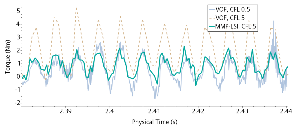
The grey curve shows the resolved VOF as the baseline simulation, the oscillatory behavior is due to the gear teeth passing frequency. The dotted line shows what happens as we increase the CFL number to 5 with VOF. The predicted torque is much too high due to the increased drag of the numerical mixture. So, what about MMP-LSI? This is the green line representing a CFL of 5. Here we have a good agreement with the resolved VOF, but over 5x faster! More efficient simulation of traditional VOF applications is not the only benefit of MMP-LSI however…
Not just broken barriers – capture previously elusive multiphase flow physics
Whilst MMP-LSI can be viewed as VOF+, its ability to capture mixtures and free surfaces in the same simulation allows us to model a range of multiple regime multiphase flow applications that were either difficult or impossible to model previously.
One such application is the multiphase pump. These are common in the oil and gas industry where oil and natural gas can be present in the same pipeline, or in water systems were air may become entrained in the system and clog pumps. This is a problem as the gas tends to form larger pockets as it separates under the body forces, particularly at off design conditions. The air can then become trapped, unable to navigate the large pressure gradients set up by liquid phases three orders of magnitude denser and forms a gas lock.
Such an example is shown in the animation above. A homogenous mixture of 90% water and 10% air enters the pump. The body forces due to the rotation of the blades causes the mixture to separate into air and water. This is only possible with the slip modeling that MMP brings to MMP-LSI. Bubbles then form on the suction surfaces of the blades, which grow and break free. These then migrate to the hub and combine to form a larger blockage that will eventually stop the pump from working altogether. These larger bubbles can only be captured with the large-scale interface modeling of LSI. MMP-LSI allows these two phenomena to coexist, and new aspects of physics such as this to be simulated.
As breaking through the sound barrier opened up new opportunities to cross the Atlantic in record times, breaking through the Courant barrier allows us to simulate multiphase flow applications more efficiently, whilst making other previously unachievable applications, reality. This and many other exciting new features can be at your fingertips in a matter of days this fall in Simcenter STAR-CCM+ 2020.3.
Keep tuned for some of the other great enhancements coming in this release.


