Locating Mid-Surface Gaps in Simcenter Femap

By David Haag and Anthony Johnson

Editor’s Note: This article is part of a series of articles by David Haag of Haag Enterprises, an advanced digital engineering shop specialized in delivering product development and industrial equipment and automation services.

A trophy truck, also known as a Baja truck or trick truck, is a vehicle used in high-speed off-road racing. This is an open production class and all components are considered legal unless specifically restricted.

_{Figure 1. Images courtesy of Hall Designs. The truck was designed for Lafortune Racecars and their customer Jeff Proctor of Honda Off-Road Racing.}

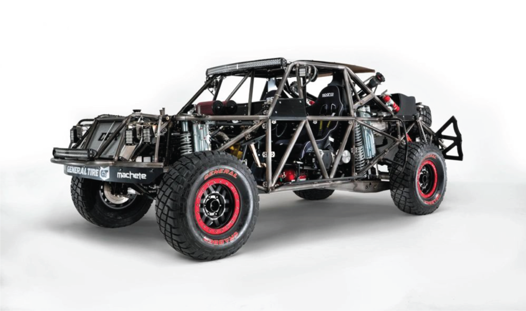
Most of the suspension components on a Trophy Truck are comprised of sheet metal weldments crafted by artisans of the industry. When designed properly, this approach will produce a stiff, light weight structure.

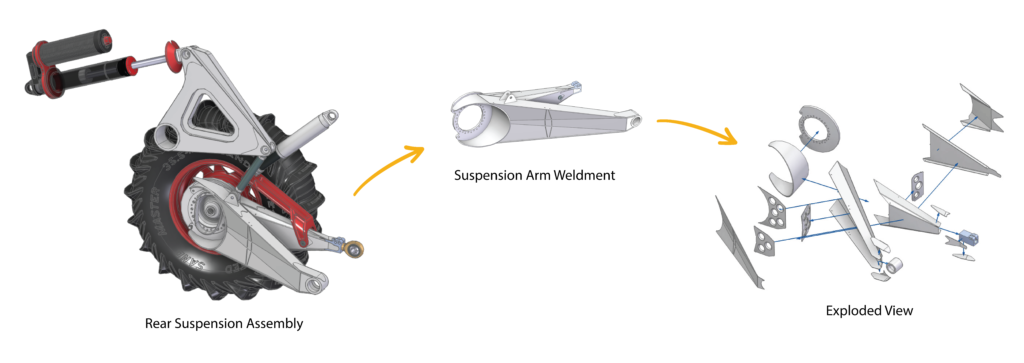
Hall Designs is one manufacturer that takes this approach, as you can see in Figure 2 below, where the Rear Suspension Assembly has been progressively isolated to show the 19 parts that make up the Suspension Arm Weldment, 17 of which are thin sheet metal parts that are lasered, formed, and then tig welded together.

Figure 2. The Suspension Arm Weldment contains 19 parts (2 machined and 17 sheet metal parts). CAD files courtesy of Hall Designs (fabricated suspension) and Camburg Engineering (coil over shock absorber).

The Mid-Surface Gap Challenge

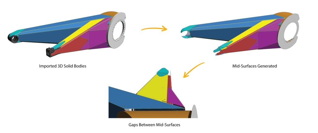
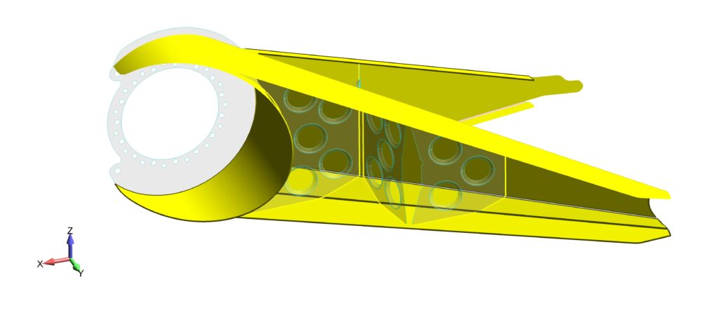
To analyze the Rear Suspension Arm Weldment using FEA, the thin-walled parts are converted into mid-surfaces, which have zero thickness and as a result, introduces gaps between adjacent components, as shown below in Figure 3.

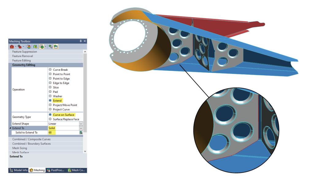
Figure 3. The thin wall plates are converted into mid-surfaces, which introduces gaps between T-junctions and the mating scab plates.

Herein lies the challenge for the simulation engineer, as these gaps must be bridged to properly transfer loads between adjacent component nodes. Figure 4 shows the common strategy for connecting gaps at T-junctions by extending surface edges to intersect with adjacent surfaces. Using the Meshing Toolbox -> Geometry Editing -> Extend command, the red curves on the gray part are selected and extended to the blue sheet solid, which simultaneously imprints a curve where common nodes will reside when meshed. While these steps are not difficult, it becomes a challenge for high component count assembly models to (1) locate the T-junctions and (2) keep track of which have been fixed.

Figure 4. Using the **Meshing Toolbox** > **Geometry Editing** > **Extend** command, the red curves on the gray part are selected and extended to the blue sheet solid, which simultaneously imprints a curve where common nodes will reside when meshed.

A quicker method for locating and connecting mid-surface T-Junctions

The Mesh Control Explorer toolbar in Simcenter Femap helps automate the process of mesh propagation between solid bodies and surface solids that lack coincident edges. We can also use this tool to find T-Junctions between surfaces, which will be our focus in the proceeding.

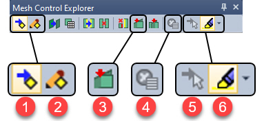
Figure 5. The Mesh Control Explorer Toolbar with magnified commands buttons and reference numbers.

In Figure 5, I added reference numbers for commands used in our workflow of identifying T-Junctions within the mid-surface sheet solids, so lets dissect the toolbar and later will discuss some example workflows.

Command reference

1. Toggle Toolbar On/Off

This toolbar can be toggled on and off at any time when meshing a model. When off, the options and settings are ignored during mesh operations.

2. Mesh Sizing Propagation Options

Limit Selection – Controls which solids/surfaces are considered when mesh sizes are updated. When using Selected Solid Only, click the Select Solids button to select solids, sheet solids, and general bodies using the standard entity selection dialog box.
On Solids – If Slaved and Mapped Surfacesis enabled, then slaved surfaces with mapped mesh approaches are considered when determining which edges to update, otherwise they are not considered.
Edges to Pair – These options will automatically find neighboring edges of “unstitched” geometric entities (i.e., individual surfaces, sheet solids, and/or “non-enclosed volume” portions of general bodies) and attempt to match mesh sizes across the multiple coincident edges.
Edge Pairing Tolerance – This is the tolerance used to automatically “pair” coincident edges. Automatic uses the default node merge tolerance, while Specified uses value provided by the user.

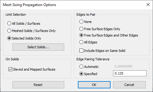
Figure 6. Mesh Sizing Propagation Options used for our Rear Suspension model.

For the Rear Suspension model, I used the Selected Solids Only and chose the components that have gaps between T-Junctions. No slaved or mapped surfaces have been defined, so that check box will have no effect in our example. The sheet metal in our weldment is .090” thick, so a gap of .090” (half material thickness * 2) should be present between edges, so I set the edge pairing tolerance to .125” to ensure we capture all edge of interest.

3. Show Edges that are Adjacent to Surfaces with no Imprinted Edge

This command will visually highlight all edges that are adjacent to a surface face, that fall within the specified Edge Pairing Tolerance, as shown by Figure 7; however, you must first turn on highlighting (#6 in Figure 5).

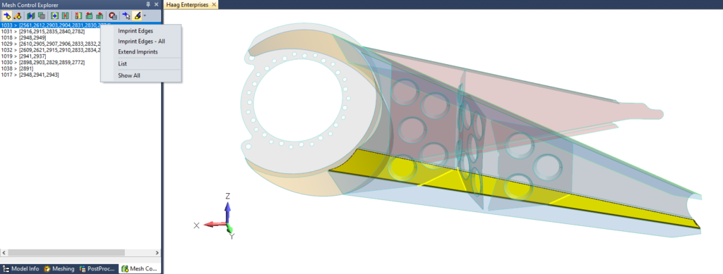
We drill down and assign actions to the pairs of interest. Notice in Figure 8, a list of each paired curve is displayed below the toolbar and each line can be selected from the list, which highlights the respective paired curves in the graphics area, giving the user instant visual feedback. A list of actions and options are available by right-clicking in the list area and function as follows:

Imprint Edges (action) applies only to the selected pair and will “burn” the curve/edge onto the adjacent surface, see Figure 8.
Imprint Edges- All (action) will “burn” each curve/edge found within the entire list onto it’s respective adjacent surface, see Figure 8.
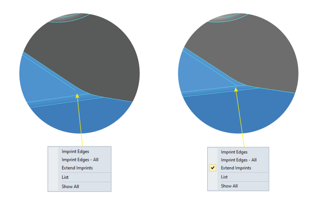
Extend Imprints (option) allows the imprinted edge to extend and terminate at the next curve within it’s path, see Figure 9.

Figure 7. By selecting the **Show Edges that are Adjacent to Surfaces with no Imprinted Edge** command, based on the Selected Solids from Step 2, the paired edges that meet the criteria are highlighted and displayed as a list under the **Mesh Control Explorer** toolbar.

Figure 8. A list of actions and options is available by right-clicking in the list area. **Imprint Edges** will “burn” the curve/edge into the adjacent surface of the selected pair, whereas **Imprint Edges – All** will “burn” all curves/edges within the list into the respective adjacent surfaces.

Figure 9. The difference between the option of Extend Imprints being checked or unchecked is visually demonstrated here.

4. Clear Mesh Control Explorer List

Not much explanation needed here, as it simply clears the list of pairings.

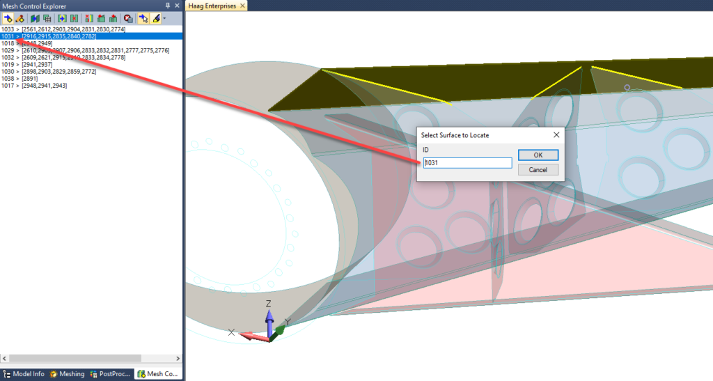
5. Select Entity to Locate in List

The show all option is nice for a high level overview, but when its time to work on specific pairing, we need a quick way of selecting from the list, especially if the list is long. Using this command (#5 in Figure 5), we can then select a face from the graphic area and the pairing will highlight within the list, as seen in Figure 10.

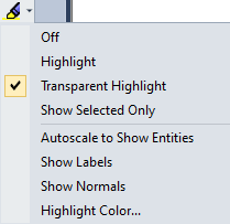
Selecting a face from the graphic area — Figure 10. By selecting a face from the graphic area, the pairing will highlight within the list.

6. Show When Selected

Contains several options to show the entities currently highlighted in the Mesh Control Explorer in the main graphics window. Only Curves and Surfaces can be “shown”, and which type of entity being shown depends on which tool was used to populate the list in the Mesh Control Explorer. By default, this command is enabled.

Figure 11. **Show When Selected** options can be accessed by clicking the arrow to the right of the button.

Example workflow and key takeaways

How we choose to model the T-junction gap depends on the ramifications if engineering changes should occur after the finite element model has been completed, which I briefly discuss and demonstrate in video.

For my example workflow, I chose to use the Mesh Control Explorer as a visual check to ensure that I have closed all T-junction gaps using the Extend command in the Meshing Toolbox, which will Imprint Edges by default. Therefore, I won’t be using the Imprint Edge actions from the right-click menu, as it did not work as planned with my geometry (it produced dual imprint lines in some instances). After extending all surfaces to eliminate T-junction gaps, we can verify using the Show Edges that are Adjacent to Surfaces with no Imprinted Edge (#3 in Figure 5) and if no results are listed, then each of the intersections have been paired by proximity and when meshed will share common nodes between the meshed surfaces.

One key takeaway for using Mesh Control Explorer is that we no longer have to create Non-Manifold bodies prior to meshing. The benefits of doing this are:

If changes occur, no need to recover manifold geometry, add new geometry, non-manifold add again.
If contact regions have been defined, when doing a recover manifold geometry, sometimes the selected faces loose associativity and it causes more work to fix.

After reading this post, I hope you find productivity gains. And I would love to hear your feedback in the comments below or feel free to email me at info@haagenterprises.com.