Getting better heat transfer coefficients for the thermal whole engine model

By Zouya Zarei

One of the questions we hear most often about gas turbine engine design is, “How can I correctly and efficiently capture convective heat transfer in the thermal Whole Engine Model (WEM).” The challenge boils down to how to ensure you are working with the correct heat transfer coefficients (HTC).

It can be a long and costly process to get HTC values because the process requires extensive experience, testing, and validation. You might be tempted to make assumptions about HTC values. But no matter how well-informed those assumptions are, there’s no guarantee. This represents a risk because local flow variations are important, and small temperature changes can have a large impact on the life of some components.

One approach to address this is to run full 3D conjugate heat transfer computational fluid dynamics (CFD) on the whole engine model, but this is computationally expensive and hence prohibitive in the early design phase where quick turnarounds are necessary. It can also be time-consuming and cost-prohibitive in the final design stages.

A “cheaper” approach to such long thermal transfer simulations is to make use of the best of both worlds: combine the aforementioned simplified thermal WEM approach for most parts of the engine with 3D CFD computations where uncertainties are the largest, in particular near cavities. We’ll explore this combination approach in this blog.

What’s the solution to whole engine model CFD?

Our primary goal remains to more accurately capture the thermo-mechanical effects on the whole engine for full mission cycles. With that in mind, let’s review the key steps to easily incorporate 3D CFD for specific regions into the whole engine model.

The following example assumes that a classic thermal WEM model already exists and has been properly setup (i.e., condition sequences, 2D axisymmetric and plane stress elements possibly connected to 3D geometry, thermal voids, streams and convective zones, rotation, fluid effects modeled with 1D elements, etc.). Ideally, this model is already validated numerically and physically, displaying a reasonable temperature profile based on provided thermal correlation approximations.

Step-by-step approach to 3D CFD of thermal WEM models

Add 3D fluid domains into the WEM

The first step is to add the fluid domains using a powerful set of advanced geometry, meshing, and mesh editing tools within the integrated Simcenter 3D environment.

In the video below, we show how to create the fluid domain representing the cavity between the stator and the rotor. The Sketch capability is used to generate a 2D profile of the cavity, guided by the edges of the components in the assembly. Straight lines and arcs form the bulk of the sketch. Curve tools like Trim and Extend ensure that the sketch ends up as a closed loop. Rotating the 2D profile then produces a 3D slice. Then trim the slice to the correct dimensions and subtract the intersecting solid portions.

As you can see, in a few easy steps the fluid domain is now ready.

The next step is to mesh the fluid domain. Since the two planar surfaces on either side are effectively periodic boundaries, identical meshes are needed on them. This is achieved using a 2D seed mesh on one face and a 2D dependent mesh on the opposite face. The next step is to mesh the domain with use 3D tetrahedral elements and assign air as a material.

Add the relevant physics

The starting point being an already existing whole engine model with all the thermal convective boundary conditions defined, to incorporate the 3D fluid domain with all relevant physics it is necessary to:

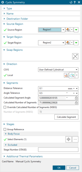
Define the periodicity of the fluid domain using the Cyclic Symmetry simulation object. Select the corresponding periodic faces and then the software automatically computes the segment angle [when using the auto-calculated number of segment option]. Since the number of segments should be an integer, revolve each flow domain with an angle that needs 360° divided by that integer.

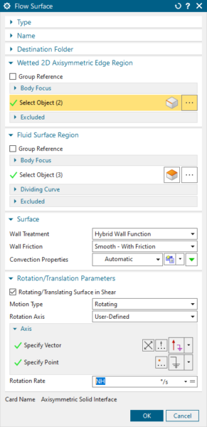
Define the periodicity of the fluid domain using the Cyclic Symmetry simulation object

Define the convective connection between the 2D axisymmetric solid and the fluid faces via the Axisymmetric Solid Interface, where the edges of the axisymmetric solid and the corresponding fluid faces are selected. In the case of the stator, since the fluid domain has a rotating frame of reference defined on it, define a counter-rotating surface to represent the stationary surfaces of the stator. For the rotor, the surface rotates in the same direction as the rotating frame of reference so no rotation needs to be defined in the flow surface simulation object.

Define the convective connection between the 2D axisymmetric solid and the fluid faces via the Axisymmetric Solid Interface

Define the connections between the 1D fluid network and the 3D fluid domain via the Ducts/Streams Junction to 3D Flow junction. Select the participating fluid faces and choose the connected streams/ducts from the available ones. It is also possible to create streams and ducts on the fly. The junction also requires specification of the type of connection, namely whether it is an inflow or outflow junction and whether the solver is required to compute the mass or pressure transfer.

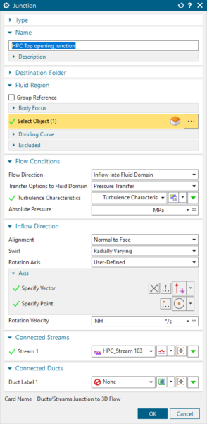
Define the connections between the 1D fluid network and the 3D fluid domain via the Ducts/Streams Junction to 3D Flow junction

Note that if the “Mass Flow Transfer” is assigned on a fluid domain having a cyclic symmetry, the mass flow value sent to the fluid domain will be divided by a factor equal to the number of cyclic symmetric segments. Reciprocally with the “Pressure Transfer” option, the mass flow value sent by the fluid domain to the ducts/streams will be multiplied by the number of cyclic symmetric segments.

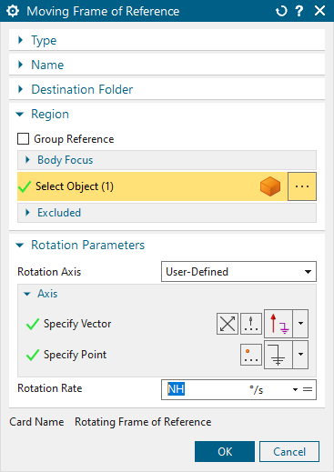
Take into account the rotation of the fluid domain using a Rotational Frame of Reference (RFR)

Take into account the rotation of the fluid domain using a Rotational Frame of Reference

Solution setup

Solving a coupled 1D-2D-3D thermal flow problem requires that you pay particular attention to the solver setup. The goal of this blog is not to provide a complete technical explanation of the recommended solution setup — this will soon be published in the form a detailed whitepaper — but the most important aspects that need particular attention are:

Turbulence model
Freeze flow
Thermal automatic time stepping
Flow convergence pseudo-time stepping
High-speed flow option
Flow convergence criteria
Transient thermal convergence criteria
Thermal-flow convergence control

Final steps and postprocessing

Once completing the model set up, the rest of the steps are exactly the same as explained in these two blogs:

The only difference lies in the postprocessing. Most of the result sets and postprocessing tools are the same (2D/3D solid temperature together with 1D fluid temperatures or flow rate), but some additional ones are available: 3D fluid velocities and temperatures, as well as local computed heat transfer coefficients that are shown in the video below. In this example local temperature variations due to the thermal interaction of the solid and fluid across complex geometry interfaces are visible. A close look at the local HTC in the cavity of the high-pressure compressor demonstrates this local variation and plotting the time-varying HTC for a few representative points illustrates this as well.

Get better predictive data

In summary, using the powerful tools in Simcenter 3D, it is possible to meet the challenges that engine manufacturers face today:

Get better HTCs by incorporating 3D-CFD into the whole engine model.
Strategically add 3D-CFD to sensitive portions of the whole engine model. This way, we get more precise results without incurring prohibitively high computational costs.
Account for local variations in flow conditions that can then provide better heat transfer predictions.
Identify temperature changes that can have a large overall impact, particularly in areas that are otherwise difficult to test.

Simcenter 3D can help aeroengine manufacturers get better predictive data for their products. It is a unique and complete platform that offers all the necessary tools to achieve efficient turbomachine simulations.

Powering up complexity

In a blog series from our partner, Maya HTT, they demonstrated how Simcenter 3D offers an integrated simulation environment for quickly and efficiently assessing thermo-mechanical whole engine responses of turbomachines. This helps ensure systems and components remain safe and achieve the best performance, even under high stresses and temperatures. These blogs also showed how the design and development process can be as seamless, error-free, collaborative, and efficient as possible to reduce costs and development time.