A magnetic field is created due to a flow of charges. That magnetic field ‘flows’ around the direction of the charges as per the ‘right hand rule’. When a voltage drop over a conductor is imposed at time t = 0, the magnetic field grows in strength resulting in a slow down in the rate at which the current stabilises.  Once the current settles to a constant value (a direct current (DC)), although the magnetic field still exists, it is not changing in time and so has no subsequent effect on the current.

In the case of an alternating current (AC), where the imposed voltage drop varies sinusoidally from +ve to -ve values, the magnetic field is always changing and thus has a persistent resulting effect on the current flow within the conductor. A so called ‘skin effect’.

DC Uniformity

Let’s first look at the attractively simple case of DC, the Joule Heating that occurs due to the electrical losses and the resulting temperature distribution within a rectangular cross section conductor. Simcenter FLOEFD is used with its capability of modelling electrical, electromagnetic, thermal and fluid behaviours all within a single simulation.

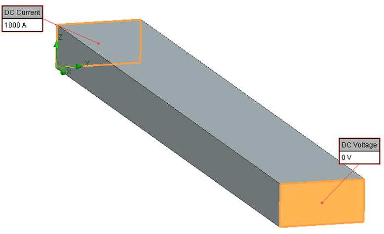
A 50mm x 25mm rectangular cross section 400 mm long Copper bar has a current of 1800A introduced at one end with a fixed 0 Voltage at the other. The bar is horizontally mounted, free floating in free air.

A steady state Simcenter FLOEFD simulation predicts the distribution of current and Joule heating power density within the bar, the resulting temperature variation both within the bar and in the surrounding air as well as the natural convection air flow that cools the bar.

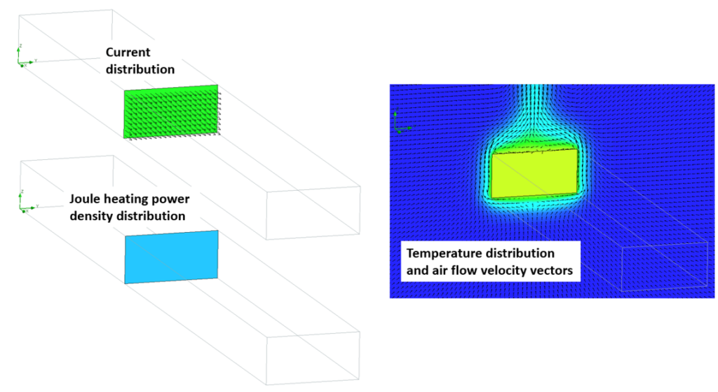
A central vertical cut plane is used to plot these simulated properties. The current distribution across the cross section is uniform, therefore the Joule heating (I²R) power loss is as well and so unsurprisingly the resulting temperature variation within the bar is very uniform. So far, so simple!

AC Complexity

Taking the same Simcenter FLOEFD model, let’s now apply an alternating current at the end of the bar.

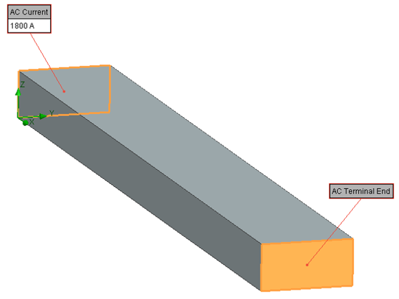
The AC current is imposed as an RMS value, the average value considering its sinusoidal variation, the oscillating equivalent current to the steady state 1800 A value. It is also set to vary at frequency of 100 Hz (the imposed voltage that is causing that AC is going from a +ve to a -ve value 100 times a second).

There’s a lot more going on in the AC case compared to the DC one! Let’s break it down a bit…

Changing B Field

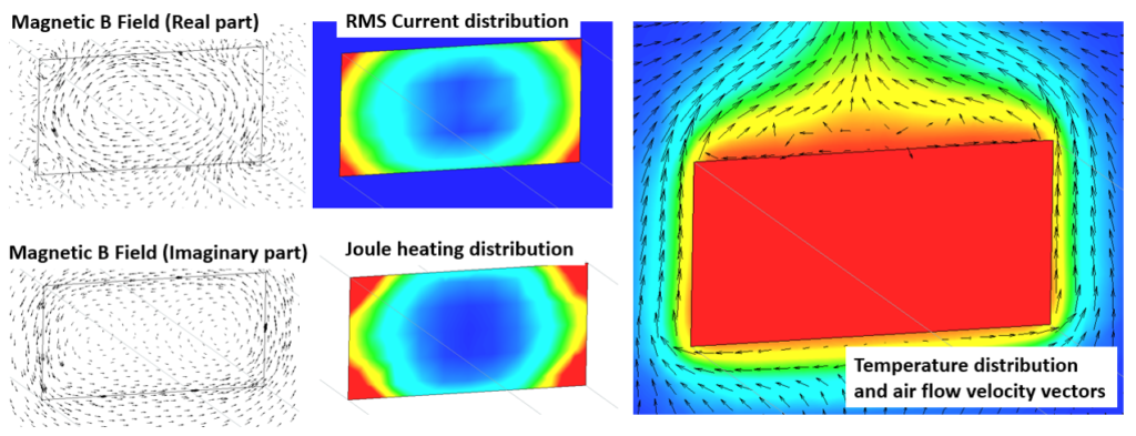
The magnetic flux density (B) field varies in both direction, shape and time as the current alternates. At one point in time it’s flowing in a kind of clockwise direction within and around the bar, at another point in time it’s flowing in an anti-clockwise direction. The 2 B field vector plots show the magnetic flux at 2 time points in a cycle, separated by 90°.

The fact that this B field is changing in time induces a back Electro Motive Force (EMF), a force on the charges, in the opposite direction to the direction the charges were moving so as to cause the changing B field in the first place. The key point is that this back EMF is greatest in the center of the conductor. So great so as to ‘cancel out’ the movement of charges there. The only place left for the imposed current to flow is therefore towards the periphery of the conductor.

RMS Current and Joule heating Fields

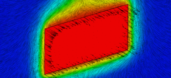
Looking at the RMS Current Distribution image shown above, the blue area of the very low RMS current in the middle of the conductor is due to this cancelling out effect. The red areas of much higher current flow, especially at the corners of the rectangular cross section, is where most of the imposed current therefore has to flow.

Current flow results in a Joule heating. Where the current density is high, the Joule heating power density will be very high (proportional to current density squared).

Temperature Distribution

With so much power being dissipated in the periphery (in the ‘skin’) of the conductor, why is the temperature so uniform? Why isn’t the temperature distribution proportional to the Joule heating distribution, i.e. higher at the peripheral edges and especially at the corners?

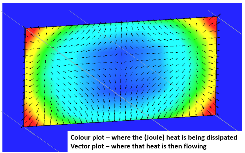
Copper is a really good conductor of heat, it has a very high thermal conductivity. Heat flows so readily through the solid it results in a near-uniform resulting temperature distribution, even at the surface where heat is transferred to the surrounding environment

Any sharp angled bends in the conductor would cause the current to crowd even more at the inner corner of the bend. This would increase the local Joule heating power dissipation which might result in noticeable increases in local temperature, especially if the conductor had a lower thermal conductivity. Extremely difficult to predict analytically, it’s a great example of the use of simulation to identify the risks associated with busbar design for example.

Skin Depth

In retrospect it would have been simpler to use a circular cross section conductor to demonstrate skin effect! The peripheral biasing of both the rms current flow and Joule heating distribution would have shown a constant ‘depth’ around the periphery, not bunched up in the corners as in the rectangular cross section example.

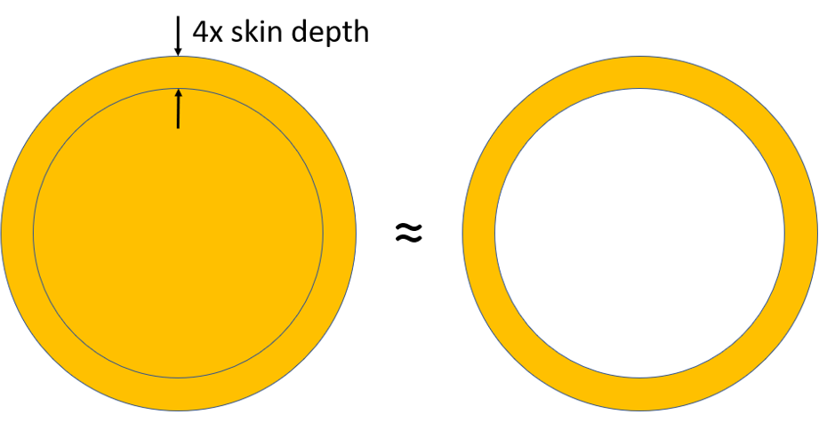
The skin depth is formally defined as the outer annular thickness of a circular conductor where 1-1/e (~63%) of the total current flows. At 4x the skin depth, over 98% of the current will flow in that region. The rest of the insides of the conductor become redundant. In fact the conductor becomes equivalent to a tube of wall thickness ~4x the skin depth:

Why Skin Depth is a Bad Thing

With all the current being forced to flow in an annulus on the periphery of a conductor, its effective cross-sectional area decreases. As the area through which the current flows is reduced, the effective electrical resistance of the conductor increases and so the voltage drop and resulting Joule heating losses also increase.

Compared to the DC case, in the bar example the total Joule heating power increased by 83% and the temperature rise by 60%, despite the same current being carried.

Skin Depth as a Function of AC Frequency

The faster the AC oscillates, the greater the rate of change of the magnetic flux density in time, the more the current is forced towards the periphery of the conductor, the smaller the skin depth becomes and the bigger the effective increase in electrical resistance, Joule heating loss and temperature rise.

A common approximation for the skin depth, δ, is:

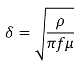
Where:

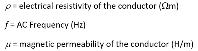
The skin depth is therefore proportional to . Double the frequency and the skin depth decreases by 29%.

Conductor Sizing and Types

For a solid conductor, you’d want the skin depth to be the same as the conductor radius. That way there’s no ‘unused’ central part of the conductor and you’ll minimise the increase in effective electrical resistance. The required radius is therefore predominantly a function of the AC frequency it will carry.

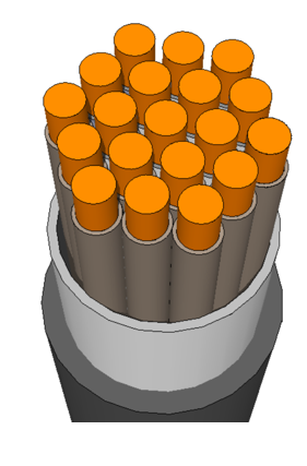
Take that one step further and bundle together many conductors, each one with a radius less than the skin depth and each one insulated, then you can carry additional current ‘in parallel’. This is the basis of a Litz wire:

Alternatively, accept that the central portion of a large cross section conductor is redundant and just use a tubular construction. Although difficult to bend and suffering from mechanical sagging over longer spans, a massive saving in weight can be realised.

Or, fill the middle of the tube with something like steel which, although not a good conductor (it doesn’t need to be, there’s little current to carry in the middle) is very strong. Longer unsupported spans can be achieved which is why Aluminium conductor steel-reinforced cable (ACSR) is a common approach for overhead powerlines.

Anecjoke

Although he was not the first to observe the skin effect, Oliver Heaviside generalised a description of it for any conductor shape in 1885. Although his formal education ended at age 14, he was to go on and make some of the most important contributions in the field of electromagnetics, mathematics and communications in the nineteenth century.

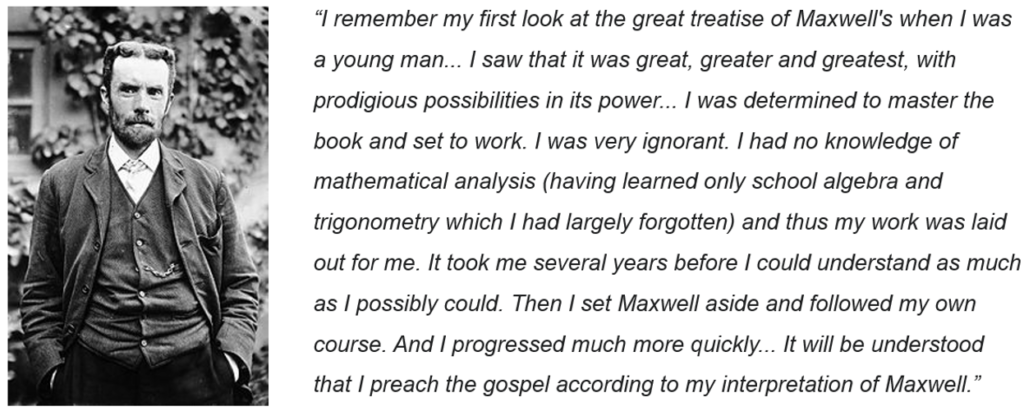
In 1884 he recast 12 of Maxwell’s original 20 equations down to 4 differential equations using more modern vector notation. These today are what we now consider as ‘Maxwell’s equations’.

In addition, he patented the coaxial cable, developed the transmission line model and from that the telegrapher’s equations, invented the Heaviside step-function, predicted the existence of what later was dubbed the Kennelly–Heaviside layer in the ionosphere as well as coining the terms: conductance, impedance, inductance, permeability, permittance (now called capacitance), permittivity and reluctance.

He died on 3 February 1925, at Torquay in Devon, receiving wider recognition of his contributions only posthumously.