Reduced Order Model for simulation speed-up with Simcenter Amesim

Reduced Order Models for simulation speed-up applied to a regional aircraft turboprop and its integration into a flight performance model.
Motivations
If you are in the system simulation business, I’m sure that at a given point in time you have been confronted with unsatisfactory run-time performance of simulation models. Due to the multi-disciplinary and mixed-fidelity nature of systems simulation, it is not always straightforward to understand how to improve models’ run-time. Sometimes, this can turn into a frustrating experience. In this article, I’ll try to explain what the most common causes of slow simulations are, and how to use Reduced Order Model for simulation speed-up.
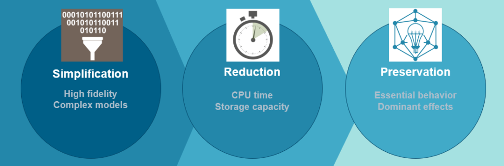
A Reduced Order Model (ROM) is a simplification of a high-fidelity static or dynamical model that preserves essential behavior and dominant effects, for the purpose of reducing solution time or storage capacity required for the more complex model.
Root causes analysis
We can usually traced back disappointing run-time performance to two root causes:
- The model is not adequate for the simulation analysis. To understand this statement, let me remind you that models are abstract representations of real-world systems. They are not exact representations, and therefore, do not produce perfectly representative results. However, the goal (and the challenge) of modeling is to include the pertinent representations necessary for the model’s intended purpose. It is logical that if the model is unnecessarily too detailed for the analysis, its run-time may be perceived as too long. If this is the case, we should consider and adapt the model to the analysis to be made.
- If, on the other hand, the model is conceptually adequate, i.e. it does not over-represent the system to be analyzed with respect to the analysis requested, trade-offs between accuracy and run-time efficiency can happen due to computational resources limitations. This is particularly true for real time applications, where we require simulations to be performed with a fixed time step. In this case, Reduced-Order Model (ROM) techniques can be useful to simplify these models preserving their essential behavior and dominant effects, with the purpose of reducing simulation time.
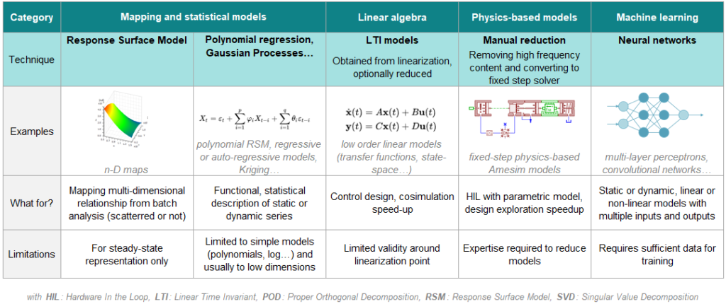
The table in Figure 1 presents ROM techniques commonly applied to systems simulation, along with some guidelines and limitations.
In this article, I’ll walk you through the applications of ROM techniques, namely manual reduction (physics-based models) and neural networks (deep learning), to reduce the simulation time of a gas turbine performance and its integration into a flight performance model.
Practical application of Reduced Order Models
The latest Simcenter Amesim release (v2020.2) comes with two new demonstrators of a regional transport aircraft and its hybridization for flight performance analysis. As depicted in Figure 2, this is accessible from the “Aerospace and Defense” section under the “Integrated systems” category.
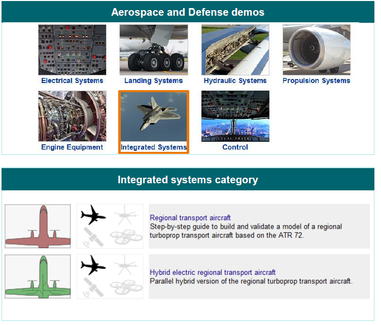
Four parts compose the model of the regional aircraft. These are: flight dynamics, controls, flight mission, and powerplant.
Having a look at the run statistics, the flight performance model takes about 1 min to simulate a mission of around 1 hour and a half. We used a regular laptop, using a GCC 64bit compiler and a variable time step (Simcenter Amesim standard integrator).
Now, despite it is actually a good run-time for a single run, it is useful to improve it, especially if the model has to simulate the aircraft performance at hundreds of points of its flight envelope.
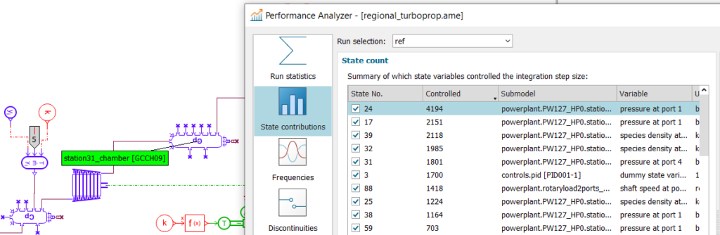
A good starting point is to look the Performance Analyzer (Figure 3). It provides a summary of which state variables controlled the integration time step. It clearly indicates that the top state contributors belong to the powerplant, in particular to the turboprop model.
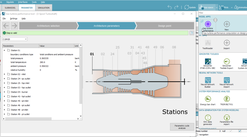
We used the Gas turbine performance tool to create this. Starting from parameters describing the thermodynamic cycle of the engine for a given design point, the tool automatically generates a Simcenter Amesim model using the Gas Turbine library components. You can launch the tool clicking on the app space menu as shown in Figure 4.
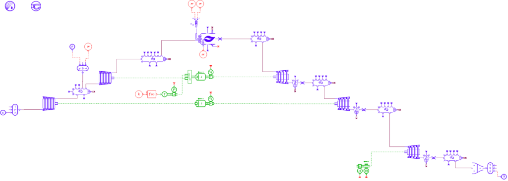
As explained, the so-generated model is the main consumer of CPU resources. For this reason, I will go through its run-time performance of turboprop model, named baseline hereafter, considered separately from the integrated flight performance model. Then, we will apply the ROM techniques with the goal to improve them.
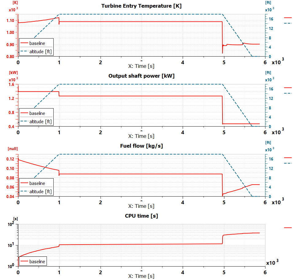
Figure 5 depicts the baseline model and Figure 6 shows a plot of the main results. The first subplot shows the Turbine Entry Temperature (TET). We plot it together with the altitude profile to help understand its evolution during the mission. The second subplot shows the turboprop shaft power together with the altitude profile. The engine controller maintains a constant power at each flight phase. The third subplot shows the engine fuel consumption. Finally, the last subplot provides the displays CPU time in a logarithmic scale.
Physical-based order reduction
A first strategy to reduce the simulation time consists in “manually” removing the high frequency content of the simulation and reducing the model accuracy keeping a reasonable error with respect to the baseline results.
We followed the following steps:
- Instead of using the NASA gas properties of the mixture definition component, we selected the linear option. This option requires a single table and simpler equations to characterize the mixture properties, differently from the NASA option. Hence, it demands less computation power to compute the mixture properties at each time step. We make this trade at the expenses of gas mixture properties fidelity.
- The reaction rate of the combustion definition was increased, passing from 107 to 105. This reduces some of the highest frequencies of the simulation.
- The model is basically composed of a sequence of resistive elements (compressors, turbines, orifices…), and capacitive elements (volumes, chambers). Making an analogy with an electrical circuit, it is possible to compute the value of the equivalent resistance and capacitance of each component (directly proportional to their volumes). This can be achieved linearizing and re-arranging the equations describing the physical behavior of these components. It can be showed that each series of resistive and capacitive elements generates an eigenvalue
, which is the inverse of a time constant
.One of the objectives of this exercise is to remove or reduce the high frequency content of the simulation. Given that high frequencies are directly responsible for the need of smaller integration time steps on the solver side. For this reason, looking at the relation above, it’s possible to reduce the frequency of the system by simply increasing the size of the volumes components. This will inevitably slow down the system response. However, performing a trade-off between the run-time benefit and the impact on the system response, it is possible to select an adequate value for the volumes. In this exercise, we increased the volumes representing the flow paths between the compressors and turbines (chambers elements) by a factor 20.
- As it can be noted from Figure 4, the combustion chamber and the turbines are followed by a sequence of orifices and volumes. These components are automatically generated by the Gas Turbine Performance tool. They account for pressure losses from one component to the other along the flow path. Keeping in mind that the goal of the analysis is to evaluate the whole aircraft flight performance, it is reasonable to assume that these losses are negligible. Therefore, the orifices and the adjacent volumes can be removed altogether. This reduces the number of state variables of the system, and the eigenvalues associated to the resistive (orifice) and capacitive (volume) elements.
- These modifications are enough to make the model real time compatible with a fixed time step of 0.1 ms and a Euler integration method. If the real time compliance is not a requirement (again, our goal is to speed up the flight performance analysis simulation), it is also possible to modify the solver settings. Carefully increasing the solver tolerance, the CPU time can improve without compromising the simulation accuracy. In this example, we increase the solver tolerance from 10-7 to 10-5.
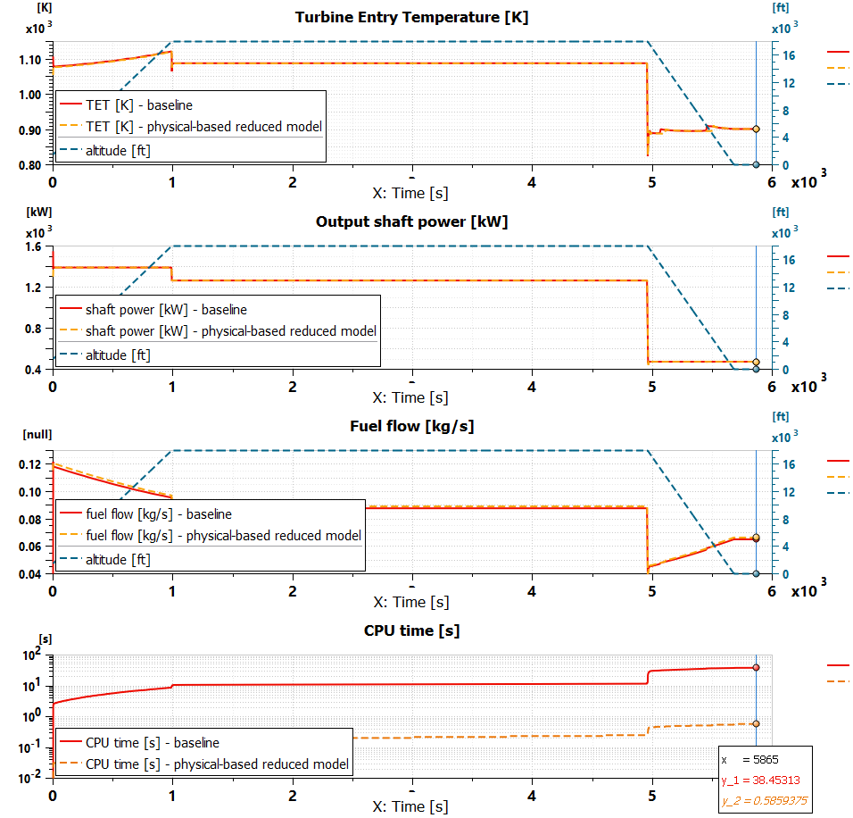
The performance comparison between the results of the baseline and the reduced order model are presented in the second subplot of Figure 6. While the differences are negligible, the CPU time was decreased by a factor of almost 70. Which is an impressive achievement with a significant CPU speed-up. The complete flight mission of 5865 s (1h 38 min) can now be executed in 0.586 s, so less than 1 second of CPU-time for 1 single run.
Deep learning order reduction
Another ROM technique consists in creating a surrogate model using a machine learning approach. Surrogate models are usually developed because of their significant performance advantage over more detailed, application- or discipline- specific (e.g., physics-based) model implementations. However, surrogate models not only take on all the assumptions and limitations of the models on which they are based, but also incorporate additional limitations from their specific implementation.
Simcenter Amesim is equipped with the Neural Network Builder, a tool capable of creating artificial neural networks from Simcenter Amesim models or external data sets. We execute 3 main steps for the creation of a neural network:
- Import of data sets for training and validation
- Definition of the neural network (inputs, outputs, hyper-parameters)
- Training and validation of the network with the data sets
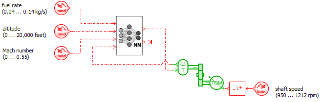
To create a consistent data set for training and validation, we modified the baseline model presented in Figure 5. The boundary conditions of the system varied randomly within a consistent range of values. These boundary conditions are altitude, Mach number (directly related to the total and static pressure and temperatures at the engines inlet and outlet), fuel flow rate, and shaft speed. These represent the model’s inputs. The outputs are the shaft torque and the temperature at the turbine inlet. Figure 8 represents the reworked model. We encaplulated the baseline model in the super-component placed in the middle of the sketch.
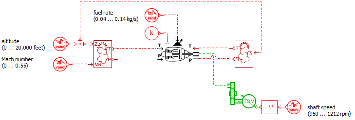
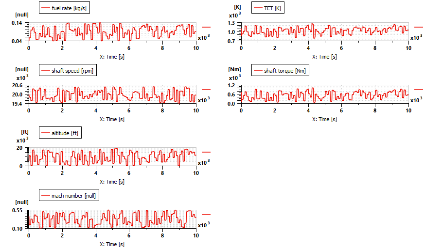
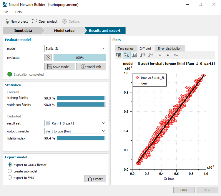
Figure 9 shows the plot of the dataset generated, with the input to the left and the outputs to the right. Given that the interest of the simulation is focused on low frequency dynamics, we selected a static neural network model to be trained. Figure 10 shows the validation step, with an overall training and fidelity index of 98%. The outcome of the Neural Network Builder is a component embedding the artificial neural network model. In Figure 11 we show how it replaces the Simcenter Amesim’s native turboshaft model depicted in Figure 8.
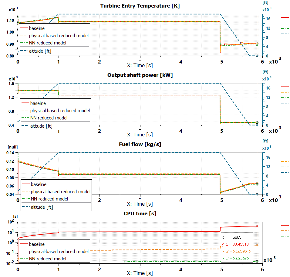
Finally, in Figure 12, we compare the results obtained with the neural network model to the baseline and the physical-base reduced order models. The neural network model tends to slightly overestimate the turbine entry temperature during cruise and underestimate it during descent. As this error is below 2% with respect to the baseline, it is deemed as acceptable. As the CPU time is reduced by a factor of roughly 2500, the complete flight mission of 5865 s (1h 38 min) can now be executed in 0.015 s. This is 15 ms of CPU-time for 1 single run. As it is extremely fast, we can now imagine launching hundreds or thousands of runs to cover the complete design space.
Flight performance model
To conclude the analysis, the physical-based reduced order, and neural network reduced order models of the engine are replaced in the flight performance model to evaluate their impact on the integrated model. We selected a high-level metric as the specific air range (SAR) to compare the performance result of the simulation models. SAR is defined as the distance traveled by the aircraft in nautical miles for a kilogram of fuel consumed. It is a synthesis of both the engine and the flight dynamics performance, making it a good gauge to compare differences between the different ROMs applied. Figure 13 shows the SAR in the first subplot (together with the altitude profile). CPU time appears in the second subplot.
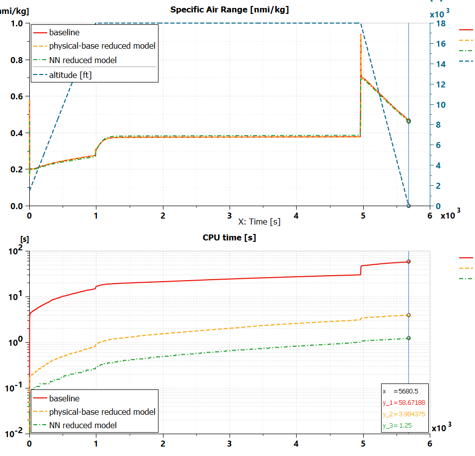
The neural network approach still presents the fastest run-time. However, its improvement with respect to the physical-based approach is less pronounced than for the turboprop engine models taken separately. We can reduce the CPU time of the integrated model by a factor of 37, against a factor of 2500 for the engine models, if compared to the baseline. The reason is that there are other portions of the integrated model responsible for slowing down the solver. It’s already a great achievement. If we’d need to have more important CPU speed-up, we would have to investigate the ROM techniques applied to the other subsystems around the turboprop engine.
Conclusion
In this article I have showed how to successfully use Reduced Order Model for simulation speed-up. We used two of these techniques to speed up a flight performance model, reworking the turboprop engine.
Each technique has its own advantages and drawbacks:
- Physical-based order reduction requires a detailed understanding of the physics modeled, the tool, and the solver working principles to be used effectively. It mainly aims at reducing the number of state variables and the highest frequencies dynamics modeled to speed up the simulation.
- Artificial neural network, a deep learning method, has a different approach. Starting from a dataset of input/outputs of a given model (system), these algorithms can trained to reproduce the correlations between those. They are very efficient from a computational point of view. On the negative side, the physics of the model they replace is not accessible. Their limitation adds up with those of the original model. Finally, their validity domain, determined by the input/output choice and the breadth of the dataset used for the algorithm training, must be respected with care.
I hope this article gave you some useful tips on reduced order model techniques and that you’ll be able to use them to speed up simulations’ run-time or make them real time compatible.
About the author:
Federico Cappuzzo is a product manager for Simcenter Amesim with the Aerospace and Defense team. He believes that system simulation will make the difference for the challenges that lie ahead for the aerospace industry. Currently, his work focuses on proving the benefits of system simulation in the fields of flight performance, hybrid-electric propulsion, and autonomous drones.
Learn more
- Discover what’s new in Simcenter system simulation solutions 2020.2 in this blog post
- Watch this video to discover how to assess regional aircraft performance with conventional & hybrid propulsion systems: