Using job distribution to optimize signal integrity analysis through parallel simulation
Job distribution with HyperLynx
Computational job distribution is an important component to scaling and optimizing any signal integrity (SI) analysis. Job distribution aims to reduce the necessary simulation time while maintaining the necessary simulation accuracy by performing calculations in parallel. These parallel simulations are completely scalable across your analysis, it can work on 3 channels, just as easily as it can work on 3,000 channels. In addition to this, it can allow for the scaling of the overall simulation accuracy. HyperLynx has specifically designed job distribution to scale throughout the skill set of the user base.
When you start to think of computation time as an available resource which needs to be balanced along with simulation accuracy and depth, you start to be able to more accurately manage and scale late-stage signal integrity demands.
It’s about time
Once your board is routed, what do you do? Do you send it directly to your fabricator, cross your fingers and hope that you got it right? As soon as your layout is complete there is often a time crunch in place that leads to a need to send things directly to your fabricator. Spending time to verify your design is something we all know that we should do, but there seems to be a balancing act between time and accuracy. There isn’t enough time to manually check everything again – after all, the rules were followed, and everyone was meticulous during routing, so the board should just work right?
Post-layout analysis, or design verification is the proper method used to determine if your design is ready to release to fabrication and its express purpose is to locate errors that exist within complicated regions of your overall design.
When looking for random errors within a design, you have to look everywhere and simulate everything.
The problem here, however, is that these errors, if present, will exist randomly throughout the overall layout. Simulating subsets of the board would result in discovering these errors through pure happenstance. You have to verify everything in this instance and you can’t do it manually. HyperLynx presents a realistic way to facilitate this.
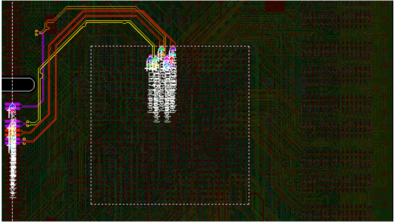
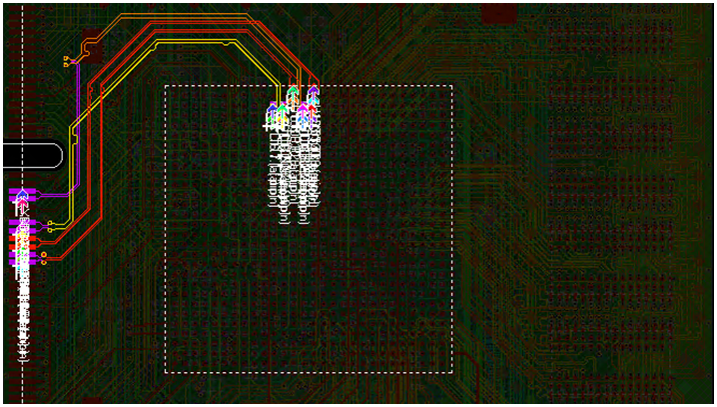
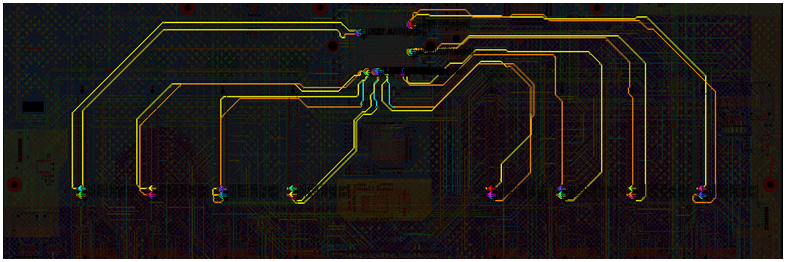
The most vital place to search for errors is within the critical nets of your design. Serial link nets are often the highest speed signals within your board and are the most likely to contain a hidden fault, making them the most critical nets to perform analysis on.
3D areas within these nets are crucial for signal integrity analysis in HyperLynx Advanced Solvers and HyperLynx Full-Wave Solvers because they allow accurate modeling of critical signal regions while maintaining computational efficiency. When full-wave solvers are applied at the system level, the entire interconnect is often too large to be practically solved in 3D. Instead, the cut and stitch method strategically segments the interconnect, reserving 3D solvers for key areas such as breakout regions, vias, and blocking capacitors.
This ensures that critical sections, including return paths and transitions, are precisely analyzed while less complex segments are efficiently represented with trace or S-parameter models. Properly defining these 3D areas is essential ensuring accurate simulation.
Evolution of job distribution
The evolution of job distribution depends upon the resources available to the individual. All of these start at the level of that user’s local machine. As the demands begin to outstrip the capability of a single machine, then the need for job distribution becomes apparent.
Local machine
You run simulations sequentially on an available local machine such as your laptop.
Remote machine
Offloading simulations onto a single remote machine is the first obvious jump from this point. It allows you to keep simulating with high accuracy while Reducing overall simulation time and freeing up computational resources on your local machine.
Multiple remote/server machines
The next logical jump is to bring multiple networked machines together and have them solve the projects in parallel either through using multiple machines, a server farm or some combination of the two.
3rd party software to handle job management.
Getting a 3rd party software solution to handle job management is the next step. These tools help allocate available resources to a job queue, removing the need to manually divide the processing between local or virtual machines. Some of these solutions include:
- Load Sharing Facility (LSF)
- High Performance Computing (HPC)
- Sun Grid Engine (SGE)
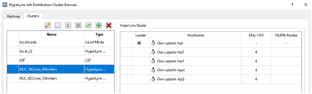
Within job distribution, the computational performance is managed through clusters. A cluster is a collection of workers with a leader. The leader will distribute jobs between the workers. Workers will perform the jobs. We use the machines created in the previous section to allocate those resources to the leader and workers A cluster can be the partial or whole number of resources of the machine. It can also consist of multiple machines, Their setup will be entirely dependent on your resources and how you choose to allocate them.
Analysis optimization
The use of local computational power doesn’t necessarily align in a logically linear fashion. As the local computational power increases, there is not necessarily a linear decrease in computational time. To demonstrate this better, I will look at a real-world example.
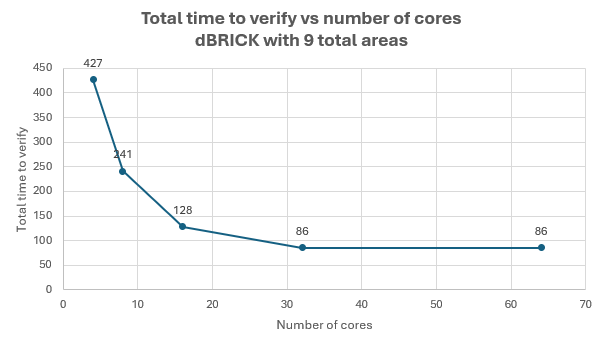
We can examine this operation by performing signal integrity analysis on one of our demo boards. This specific design is a dBRICK plug-in card which is part of dRedBox system and is widely used in many of the available HyperLynx workshops.
When run on a single local machine with 4 cores, this equates to 427 minutes of compute time. As we double the number of cores used, the compute time roughly halves, but we quickly begin to reach diminishing returns, and after adding 32 cores, our analysis time plateaus.
Distributed computing
If we expand our analysis above to include the PCIe channels on the motherboard, we end up with a much more robust job. This example includes 32 nets and requires solving 32 3D areas using the HyperLynx Full Wave Solver.
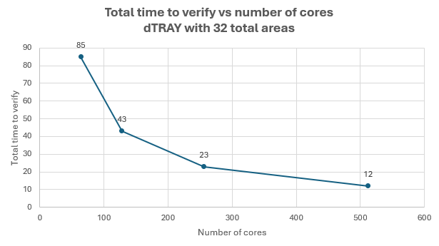
This process starts using 2 local workers containing 64 total cores and results in a baseline 85-minute compute time. As we add remote workers and double the cores provided, the computer time does not plateau. With 16 remote workers using 512 total cores, the job is brought down to just 12 minutes.
If we compare the first value in this chart with the last value in the previous chart, we are looking at the same value (64 cores) and approximately the same computer time (85-86 minutes). This demonstrates that the nature of how the job is distributed within the available processing power is an important component in the overall time to complete the analysis
Running a full system verification on the motherboard and plug-in card on a single 32 core machine would require over 18 hours of computation time, and would risk some error or interruption happing during this time. Using job distribution allows you to review the reports showing a complete PCIe full wave solver analysis for 134 3D areas and receive actionable same-day feedback in about 80 minutes.
Summary
All signal integrity analysis seems to be performed within a space uniquely susceptible to time crunches. Managing and leveraging available resources is an important component in this overall process. Balancing accuracy with turn-over time is an important component to consider when designing your process.
Ultimately, actionable data needs to be provided in a timely manner so that the feedback can be provided while it is still useful. It isn’t overly helpful to get a snapshot of your design from 2 weeks ago, these things ideally need to be loaded at the end of your work day and available when you return the next day. Realistically, working compute time needs to be compressed into 8-14 hour blocks, ideally performed overnight with results available the next morning. Larger enterprise clients find that 3-4 day compute times are acceptable for very complicated designs.
Job distribution is available for HyperLynx Signal Integrity, Power Integrity, HyperLynx DRC and HyperLynx Advanced Solvers.
Once the computations have taken place the data needs to be sorted and structured in a way that is easily and instantly discernable and readable. HyperLynx works to facilitate this with Scatter plots, interactive reports with pass/fail metrics, time domain metrics, frequency domain metrics, eye diagrams for all signals, and much more, all of which allows the designer to get both a quick overview of the general condition of the analysis as a whole, as well as the ability to quickly drill into any one data point.
Getting the best possible result in the time available.
Learn more:
Learn more about job distribution with HyperLynx and explore other Hyperscaler solutions provided by Siemens by watching the on-demand webinar: Hyperscaler design and verification with HyperLynx.