Flow Visualization and the Beauty of the Vortex Dome
The trouble with fluids is that they’re transparent. From a fluids dynamics perspective, this is problematic if you want to study their behaviour. Various flow visualization techniques exist, Rheoscopic fluids being one of the more beautiful approaches.
Transparency
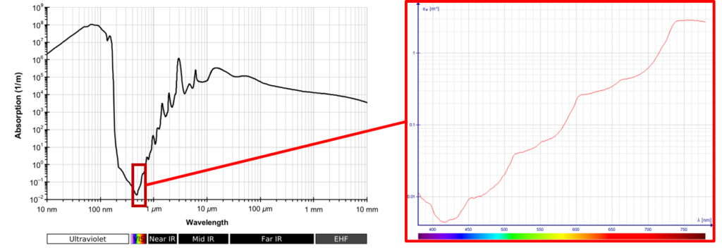
The reason fluids are transparent is due to the interaction of the photons passing through them and their atomic (or molecular) electrons. Although the physics is quite fascinating, it is somewhat out of scope of this blog. Suffice to say that some electro-magnetic frequencies pass through a liquid with little absorption or scattering, others much less so.
Considering water, the energy of the EM frequencies in the visible range is absorbed much less than the higher and lower frequencies. Not all visible colours pass through as easily as each other though, blue is absorbed least, which is why the oceans look blue.
It’s just as well visible light passes most easily through water. As our eyes are filled with the stuff there would be little to see otherwise (but sure, this is an anthropic point to make). What’s more coincidental is that the highest level of EM energies emitted by the sun are also in the visible band, or maybe it’s just that we have evolved to capitalise on it.
Rheoscopic Fluids
One way of visualising fluid flow is to introduce small particles into the fluid that themselves reflect and scatter light much more efficiently than the fluid. These particle laden fluids are called ‘Rheoscopic fluids’, derived from the Greek Rheo – ‘flow’ and Skopeo – ‘examine/inspect’.
Rheoscopic History
In 1785 Johanne Wilcke (he who coined the term ‘Specific Heat’) added burnt lime particles to visualise vortex breakdown in a stirred tank. Later Henri Bénard used graphite and aluminium flakes to visualise the now eponymous convection cells. At the turn of the 20th century Ludwig Prandtl used mica particles on the surface of a fluid to investigate flow around bluff bodies. In the 1960s the artist Paul Matisse (grandson of Henri Matisse) invented the Kalliroscope, a glass covered ‘art’ device filled with a rheoscopic fluid using Guanine particles.
Guanine is favoured as a Rheoscopic additive due to its similar density to water so that the particles do not sediment too quickly. Guanine was commonly used by the cosmetics industry to provide the reflective lustre in makeups. However with 1kg of crystalline Guanine particles produced from 50 tonnes of fish (from their shiny scales), mica is now the common alternative.
DIY Flow Visualization!
It’s surprisingly easy to make a rheoscopic fluid at home. ~0.5g of Mica powder, the glittery variety, is added to some water, et voilà!
What’s Going On?
Whereas it’s evident the particles do show up the flow patterns, it’s less clear exactly what they are showing. To understand their behaviour it’s first important to appreciate their size and shape:
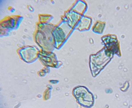
The particles are flakes of crystal, of the order of 1 micron thick and 10s of microns long/wide. Due to their small volume and thus small mass, they quickly align with the flow, rather they align based on the shear direction:
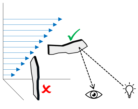
They are highly reflective and so glitter when angled between a light source and your eyes accordingly. When the flow slows, or when the shear decreases, they tend to wobble about more randomly resulting in a surface shimmering effect.
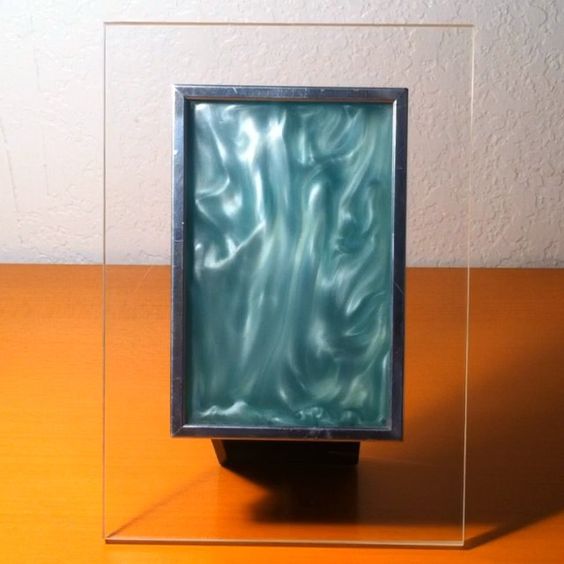
The Vortex Dome
After having seen a video of it on YouTube, I decided to buy a Vortex Dome from Physicshack, for my eldest for Christmas.
It’s the shape of a spherical cap, filled with mica laden water, mounted on a low friction bearing (the slight wobble in the video is due to the uneven table surface). The most beautiful of flow visualization Rheoscopic devices (more than just a toy), I should have bought 2 as I’ve been ‘playing’ with it more than my son has!!
Simulating the Vortex Dome
The beauty of CFD is that it ‘instruments’ a flow field at 1000s of points, unobtrusively. From that, various post-processing techniques can be used to create views and animations of the fluid dynamics. This enables much greater insight into the reasons for the observed flow than could ever be obtained experimentally, be it using Rheoscopic fluids, hot wire anemometry, particle image velocimetry, laser Doppler velocimetry, interferometry, tracers etc.
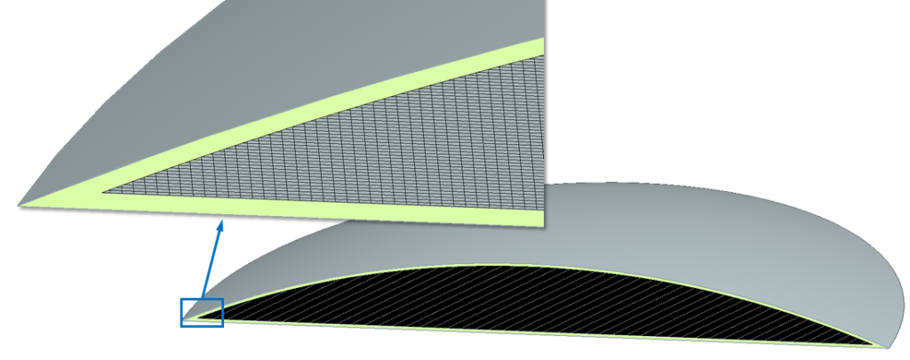
An application well suited to either Simcenter STAR-CCM+ or Simcenter FLOEFD, I opted to use the latter and constructed this deceptively simple model:
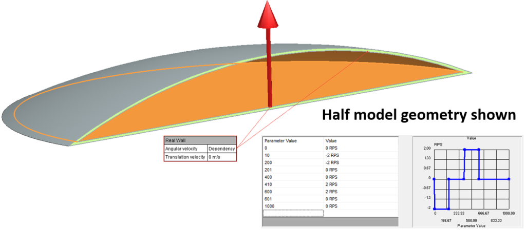
The mica particles were not modelled directly, the working fluid was set to water with a density slightly increased to account for the 5g of added mica. Rotation around the central Z axis was set on the 2 inner wall faces to 2 RPS (revolutions per second) in one direction for 1s, no rotation for 1s, 2 RPS rotation in the other direction for 1s then a final 2s of no rotation (time step of 0.005s for the eagled eyed among you).
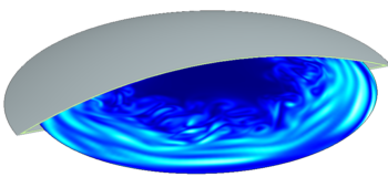
For reference, this is how the actual Vortex Dome behaves under these rotational conditions (apologies for the fat finger obscuring the view):
A horizontal plane plot, showing the transient evolution of the velocity vectors, is a good place to start to understand the overall flow behaviour:
The faces of the dome have a higher tangential velocity further away from the central vertical axis. This first spins up the fluid at the periphery. The momentum of that peripheral flow then penetrates in towards the core of the dome. The fun starts when the flow direction is reversed. This creates massive shear that generates complex vortex behaviour.
Taking a vertical slice through the centre of the dome, and plotting both velocity vectors and a contour plot of speed, provides further insight into how the momentum near the walls advects into the dome core:
Emulating Rheoscopic Behaviour
A direct simulation of a Rheoscopic fluid would entail modelling each particle, their alignment with the shear direction and a lighting model that calculated the optical behaviour for each particle in the context of the ‘view from’ location. Assuming an average particle size of 1x10x100 micron, knowing the density of mica and the total mass of mica particles, there are about 1785714286 mica particles present in the dome (roughly 😉 ). Modelling ~2 billion particles is quite intractable, at least on my laptop.
Due to the relationship between the velocity shear tensor and the orientation of a particle described above, one option is to instead plot the magnitude of a property of the flow that is related to shear. Vorticity is a good candidate:
Taking the absolute size of the Vorticity vector and plotting its distribution at each time step is about the best one can hope for in easily emulating what a Rheoscopic fluid shows.
Only remaining question is where in the dome to plot its distribution and evolution? I have chosen a curved plane 1.5mm inset from the top dome surface as a kind of mid way point of how ‘deep’ into the particle laden flow one can see. The absolute value of the vorticity does not matter, just its relative distribution, so the colour map used to plot it is normalised to the min/max extents at each time step. Blue = minimum vorticity, White = maximum vorticity.
So, looks nice enough, but how does it compare to the real thing?
Not bad. Qualitatively it’s a fair match, but there are some differences. The diffusion of momentum from the periphery to the almost stagnant central part of the dome is underpredicted slightly. You never learn anything from getting things right first time, so let’s finish off by considering ways in which the model might be improved.
Reasons to be Cautious, 1 2 3
1) Newtonian or not?
Newtonian fluids are characterised by a linear relationship between the viscous shear stress and the velocity gradient at any given point. The coefficient of this linear relationship is the fluid’s viscosity (the ability of a fluid to stick to itself). Non-Newtonian fluids however have a viscosity that itself is a function of the shear. Toothpaste is a shear-thinning non-Newtonian fluid, its viscosity decreases as the shear is increased. This is why the harder you press on a toothpaste tube, the more easily it comes out. Conversely, add cornstarch to water and you get a shear-thickening non-Newtonian fluid. You can walk on it by rapidly putting your feet down firmly enough, stay still and you sink!
Some fluids are non-Newtonian due to containing many particles suspended in a pure Newtonian base fluid. For example the shear thinning nature of blood is due to blood cells sticking to each other in stacks which tend to increase the effective viscosity. As the shear is increased, the blood cells detach, separate and the effective viscosity decreases.
There are about 2 billion mica particles in the Vortex Dome, 6000 particles per mm3 equating to about 20 particles every linear mm. With an assumed size of 1x10x100 microns, they at least would interact, possibly stack and so the Rheoscopic fluid might also exhibit shear-thinning characteristics. Unfortunately I do not have access to a Viscometer to determine non-Newtonianess and measure the viscosity. I would say though that this is the main candidate reason for the observed differences between simulation and test.
2) LES, really?
When using CFD to simulate turbulent flows it is common to adopt a ‘Reynolds Averaged Navier-Stokes’ (RANS) approach. With RANS all the turbulent vortices are considered time-averaged by the equations that are solved. Think of it as the simulation equivalent of taking a long exposure time photo. Alternatively the turbulence can be simulated more explicitly by taking a Direct Numerical Simulation (DNS) approach. Here the computational mesh cells and time steps used are small enough to resolve all the eddies, down to the smallest scales. More like a high resolution camera with a very short time exposure taking multiple pictures over time.
A half way house between RANS and DNS is Large Eddy Simulation (LES). With LES the mesh is small enough to resolve the bigger turbulent vortices, the small stuff is modelled using a sub-grid scale model (SGS). For the Simcenter FLOEFD model I used a uniform Cartesian mesh with a cell size of the order of 0.67mm:
This resulted in just over 4 million cells which just about maxed out my laptop memory and, with 1000 time steps resolving the 5s of Vortex Dome behaviour, took overnight to solve. The Kolmogarov scale (length scale at which the turbulent energy is dissipated due to viscous effects) for this model is ~100 times smaller than the mesh size used. So this model really really isn’t a DNS. Can it be considered an LES simulation? The mesh should be small enough to resolve the eddies down to some part of the inertial subrange of the turbulent energy cascade spectrum. Likely it does, but with no SGS as such to model the rest of the energy cascade (the Simcenter FLOEFD was modelled as Transient and Laminar), at most this simulation could be considered a type of ham-fisted monotonically integrated LES that relies on numerical diffusion as the SGS model.
3) Fat Fingers
Physically implementing the rotational boundary conditions on the Vortex Dome to the same accuracy as they were prescribed on the model was ‘challenging’. Using just a finger to spin up, stop, change spin direction at precisely 2RPS with 1s intervals was never going to be exact.
Insight and Understanding
Despite the above issues, the simulation had utility in that it provided insight into the fluid dynamics of the Vortex Dome, enabling an understanding of the flow. CFD circumvents many of the problems associated with flow visualization and is, by its nature, much more flexible than physical prototyping or experimentation. From a product design perspective however, both simulation and test can be used hand in hand to build better products, faster.