Response Surface and Sequential Optimisation of a Heatsink Using FloTHERM. Part 5 – Sequential Optimisation and Compound Cost Functions

Sequential optimisation is an alternative optimisation strategy that can be run in FloTHERM’s Command Center module. As with response surface optimisation, a cost function needs to be defined that captures the design intent. The optimisation will seek to identify a set of model parameters that results in a smallest cost function value. To spice things up a little we’ll consider a compound cost function and include a constraint on the model inputs.

Minimisation of heatsink mass, without compromising thermal performance, is a common design intent. A cost function that includes mass and thermal contributions can be constructed:

We retain the mod(component temperature – 85) portion but add to it the mass of the heatsink. To compensate for the different magnitudes in these two contributions (degC and kg) we can weight (not the cleverest of puns I admit) one of them to bring it into line with the order of magnitude of the other. In this case a weighting factor of 100x is applied to the mass. So, a small cost function will be one that indicates on temperature performance AND a minimised mass.

Let’s also introduce additional parameters into the mix, in addition to the TIM2 resistance, heatsink base thickness and fin height, we add number of fins and fin width:

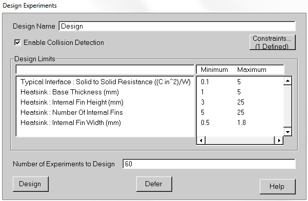
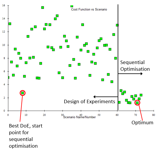
In addition we can constrain the (computational) experiments that will be created by defining a constraint rule indicating that base thickness + fin height < 15mm. As before we then create a DoE with 60 experiments, solve and note the cost function for each one.

After that a sequential optimisation can be invoked that starts from the ‘best’ (i.e. lowest cost function) experiment and automatically creates and runs a model variant that it believes will reduce the cost function.

This process is automatically repeated, each time refining the model settings, hunting for reduced cost function behaviour. In fact it is searching the local response surface gradient, identifying where the ‘bottom’ of the local cost function response surface is.

After a few sequential runs it stops and reports the optimal model:

A common question is “how can we be sure that this is a global optimum (minima)?” To answer that an extension to the DoE can be made. 60 additional experiments are created, distributed into the gaps of the existing DoE, no need to rerun the experiments that have already been solved. Again a sequential optimisation study is conducted and a new optimum found:

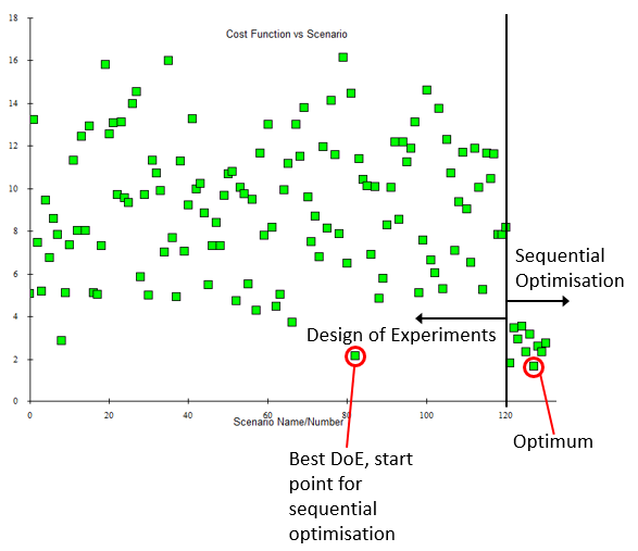In this case the same optimum was identified again. In fact, so long as the best experiment from which the sequential optimisation starts is somewhere on the sides of the lowest ‘valley’ of the response surface, the bottom of that valley will always be found.

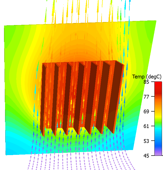
The resulting heatsink is very typical of natural convection designs, fins are very thin with large gaps between them:

And here’s a gratuitous colourful image of its simulated performance!

To finish off this series we’ll take another look at the response surface approach and show how the response surface can be used as a model, a so called response surface model (RSM).

1st March 2016, Towcester