Response Surface and Sequential Optimisation of a Heatsink Using FloTHERM. Part 3 – Cost Function Response Surfaces

A design of experiments based study will provide a scatter gun type indication of how the system performs with a user defined number of combinations of design parameters. These pin points alone might provide some insight, but, by using interpolation methods to ‘fill in the gaps’, a complete picture of the behaviour of a design can be painted. These ‘response surfaces’, when based on a parameter that captures the design intent, can allow the optimum combination of design parameters to be identified directly.

Concepts are always simpler to describe when using lower dimensions. Consider a 1D problem, where there is a single design variable. Changing that variable will result in a change to the resulting behaviour of a system. A DoE approach will result in points being created that relate the input to the output. A response surface is simply a curve fitted to those points. Such a capability is available in Excel and often used:

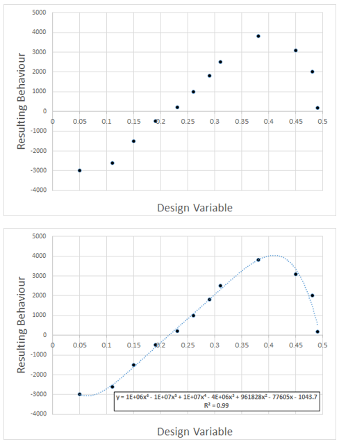
In the above example a 6th order polynomial relationship was used, the coefficients automatically determined so as to provide as good a fit as possible. The R^2 value giving a measure of the goodness of fit (1.0 is a perfect fit). When there are multiple design parameters that are being varied, things get more complex. The response ‘surface’ becomes an N dimensional object. Graphics have advanced much over the last few decades but no one has yet cracked the nut of drawing a 4+ dimensional object! From a mathematical perspective though, such surfaces can be created.

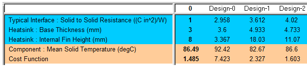
For this example we have 3 design parameters that are being varied. We now need to quantify the behaviour of the design in terms of a single metric. A cost function is so defined. It could be the resulting temperature of the component, but let’s make it a little more interesting and define the cost function as the amount by which the component is over or under temperature. We want to determine what combination of design variables will give us just the temperature we want, not over-engineered, not under-engineered. Let’s say cost function = mod(component temperature – 85 DegC). This is then tracked using FloTHERM’s Command Center, for each of the solved DoE combinations, shown here for the first few (computational) experiments:

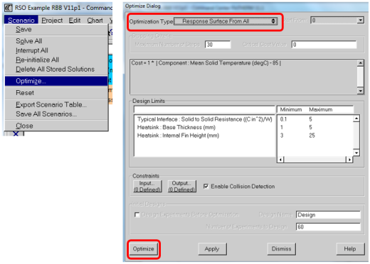
Sure, if enough (computational) experiments were created and simulated, chances are one of them would result in a cost function = zero. Generating a 3D response surface that relates the cost function to a limited number of combinations of design variables allows for the ‘lowest point’ on the response surface to be identified, efficiently. If the design space is big enough, or there are enough degrees of freedom, the lowest point is often at zero.

Creation of the response surface is straight forward in Command Center:

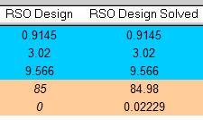From that, the lowest point on the cost function response is identified and a Command Center project is created from those optimal set of design variables. To confirm that this is indeed truly the optimal point, the response surface optimum (RSO) project is copied, 3D CFD solved and the simulated cost function returned.

Not bad! The actual simulated value was very close to the response surface predicted value (0.02 degC difference) . The reason for the difference being due to the goodness of fit of the response surface to the solved DoE points which in return is a function of the number of DoE simulations conducted. In this case 60, that’s 20 per degree of freedom. In our experience between 10-20 per (computational) experiments per degree of freedom is often sufficient enough for a good response surface fit to be achieved.

Inspection of the response surface itself provides more insight into the sensitivity of this optimum to changes in the design variables. Inspection of the response surface error indicates whether more simulations are required. Both of which we’ll look at next.

11th February 2016, Ross-on-Wye