So, you want to predict component temperatures do you? Part V
Like a river this blog series is slowing down due to its increased width and depth, that and a lot of travel on my part. So, let’s get it back on track! The previous blog focussed on the relatively well known 2 resistor compact thermal model (CTM) method, its strengths (simple to measure and describe) and its deficiencies (unconfirmed and inconsistent accuracy for different package styles and operating environments). For part V I’m going to focus on the more advanced and accurate DELPHI CTM methodology.
An EU funded research project, headed up by Flomerics with a number of other European industrial partners embarked on a 3 year project in the 90s to derive a boundary condition independent (BCI) compact modelling methodology for IC packages. A number of papers were published as a consequence of the DELPHI project, one of the formative ones being “The world of thermal characterization according to DELPHI-Part I:Background to DELPHI”. JEDEC recently (and somewhat after the completion of the project 😉 ) ratified the approach and so it now has a renewed relevance.
In essence the DELPHI approach is similar to the 2-R approach in that a thermal resistor network CTM is used to represent the thermal behaviour of an IC package without the package having to be represented explicitly. The topology of the resistor network is more complex and this is central to it’s advantage. Accounting for an increased number of internal thermal resistances within a package will more accurately capture the predominant conductive heat flow paths, not ‘shoe horning’ them all into either from die to package top and from die to package bottom.
I won’t dwell on the method used to derive the actual thermal resistance values, suffice to say that the network is numerically exercised in a number of different operating environments via imposing different combinations of heat transfer coefficient around the package surfaces. From those numerical experiments, the resistance values are determined such that the CTM will be accurate for all those environments.
The representation of a DELPHI model in a 3D FloTHERM simulation has two parts. First the periphery of the network model consisting of faces that ‘see’ the rest of the model, the PCB, the air, the heatsink etc. is defined. Then the internal network itself, whose peripheral nodes exist on the peripheral faces mentioned above.
The network topology looks like this:

The physical realization of such a network in a FloTHERM model looks like this:

(The leads node is optional in that it isn’t required for BGA type packages)
OK, that’s all well and good but what about its accuracy compared to the 2R model? To answer that lets go back to the two package examples used in the previous 2-R blog. For the 2R models one was accurate when compared to the detailed model, the other very inaccurate. If the DELPHI method of presentation was any good then it would be accurate in both cases. The following tables show the predicted junction temperature rises over ambient for detailed (i.e. correct (ok, that assumption warrants a blog series as well…)) 2-R and DELPHI methods of package representation:

The point being that DELPHI is consistently accurate whilst 2-R isn’t inaccurate as such, just inconsistently accurate.
As a reward for hanging on and getting this far here’s a sexy animation of the detailed CBGA model:

7th December 2009, Ross-on-Wye