Simcenter STAR-CCM+ v13.06: Finding the differences that make a difference…
Can you see the differences between each of the three images in the picture below?
![]()
Backing up a bit, you’re looking at the pressure contours on the bottom of an impeller in a mixing tank. Each image corresponds to a different operational condition. Looking from left to right, you see the steady state results for 270 rpm, 300 rpm and 330 rpm respectively, from three separate simulations. “Small multiples, whether tabular or pictorial, move to the heart of visual reasoning – to see, distinguish, choose.” notes Eduard Tufte (1995, p. 33)[1] in one of his seminal books on visualizing information. So, we can “see” differences with this method of visual interrogation. When it comes to choosing a better design or an advantageous operating condition, here’s the real question: In what ways do these differences matter? To answer that question, we need to combine both visual and numerical perspectives.
In Simcenter STAR-CCM+ v13.06, we’re enabling that combined perspective by leveraging our mature mapper technology, giving us a powerful method to store data within simulation (sim) files. You’ve been able to load, map volume-based simulation history (simh) results and store them in your sim files for some time now. Yet, a good rule for productive data analysis is to always work with the smallest amount of data needed to make decisions. What’s new and exciting is our ability to load, map and store surface-based simulation history (simh) results. Not only will this save you disk space and lower your resource requirements for postprocessing, you’ll be able to quantify differences for a wide range of comparative scenarios.
Let’s look again at these three operational conditions. First, we’ll choose 300 rpm as our baseline .sim file. Now, if we were to store and save the pressure in a simh file for the entire mixing tank, it would be ~515MB. Instead, we’ll create simh file snapshots for the high and low rpm operating conditions, storing only the pressure at just the impeller boundary surfaces. These simh snapshot files are very small, ~1.5MB each. Compared to the volume-based simh file, a surface-based simh file is ~340X times smaller! After mapping the boundary surface simh files, we now have simple Field Functions to reference these other operating condition pressure results within our 300rpm baseline sim file. Referring back to the starting picture at the top of this story, we were able to generate that image, showing all three operating conditions, in the same scene, from one baseline .sim file, using just one Simcenter STAR-CCM+ license. Visually informative and convenient for sure, but we still need a critical evaluation. Are these differences significant?
The last step is to create two Field Functions: 300 rpm (baseline) minus 270 rpm and 330 rpm minus 300 rpm (baseline). In the animation above, we can see that the pressure differences vary notably across each of the impeller blade surfaces. We’ve got a 10% difference in rpm versus the baseline for both cases, and the numerical differences are roughly in the same range. What is interesting is the variation of pressure over the blade surfaces – it’s far from uniform, and different for each blade. Please note: These simulation results are steady state – the impeller is rotated as a visual effect only to show the local variations over all the blades without having to change the view.
We can use this same basic workflow to examine impellers with differing blade pitches. In the animation below, we are looking at a 36 degree blade pitch, at left, and a 50 degree blade pitch, at right. Despite our side-by-side visual presentation, it’s still difficult to see the local spatial pressure differences.
This time, we define the 50 degree blade pitch as our baseline .sim file. Next, we create a simh representation of the 36 degree blade pitch case. And, lastly we use our surface mapper to store the simh pressure results in our baseline .sim file. This example takes a little more work than the previous one – we need to apply a simple transform independently to each blade and the good news is that this is well within the capabilities of our mapper.
The quantitative results presented in the animation above show clearly that the magnitude of the differences between the two blade pitch designs are significant. It’s also informative to see where the differences on the impeller are the most different. We can see exactly how much the pressure changes on the top and bottom surface of each of the impeller blades. Again, please note: These simulation results are steady state – the impeller is rotated as a visual effect only to show the local variations over all the blades without having to change the view.
We can just as easily look at differences between time steps for an unsteady analysis of our mixing tank. To look at pressure differences between time steps, we first pick a suitable time baseline. To avoid start-up fluctuations, the baseline is chosen to match the start of the third full blade revolution. In the animation below, at left, we are resetting our baseline for every 120 degrees of impeller rotation, matching the angular span between blades. At right, we reset the baseline at the start of each blade revolution to see how much the pressure on the impeller fluctuates with each full blade turn. The outline shows the starting position of the blades and serves as a useful time marker. Looking at these time differences side-by-side, we can get a sense of the magnitude and local variation of pressure on the impeller for two different time scales. These spatial and temporal layers of information give us some insight into possible fatigue issues and will likely lead us in the direction of further analyses to better understand failure risks over a wider range of operating conditions and impeller design parameters.
We’ve used our new Simcenter STAR-CCM+ v13.06 capability to load, map and store surface-based simulation history (simh) results to look at differences between operating conditions, designs and time steps. I’d be remiss here if I didn’t note that doing these kinds of operational sweeps and design variations fits very well with our existing Design Manager capabilities. Today, it is possible that we could have looked at a much broader combination of operating conditions, varying blade pitch. In short, it’s easy to generate lots of data. With our ability to store surface-based as opposed to volume-based information, we’re making it practical to store more compact artifacts that can be archived and easily retrieved for later in-depth analyses. And that makes all the difference when it comes to understanding and confidently proving which designs and operating conditions are the ones you should invest in.
You can also learn more about how Solution History (simh) can help your quantitative analyses by working with less data, please check out Less is more only when more is too much in STAR-CCM+ v12.06. To learn more about how you can benefit from using Solution History (simh) workflows with your derived parts, please check out Solution History Support for Derived Parts in STAR-CCM+ v11.04.
[1] Tufte, Eduard R., Envisioning Information. 5th edn. Graphics Press, 1995.