Experiment vs. Simulation, Part 2: TIM Thermal Conductivity
The temperature rise that electronic components attain in operation is due to 3 things. The power that they dissipate, the ambient temperature surrounding the product and the various thermal bottlenecks that the heat passes through on its journey from the source to the ambient. An accurate simulation requires all 3 aspects to be modelled correctly. In terms of the bottlenecks, conductive resistance is critical, especially close to the heat source where the heat flux values (W/m2) are high, due often to the small areas through which the heat flows. A (1D) conductive resistance is commonly characterised by the thickness of the solid object divided by its thermal conductivity times its area. Getting the conductivity correct is a must in any electronics thermal simulation.
Electronic products are highly complex assemblies of many different parts with varying thermal conductivities. An integrated circuit (e.g. on a Silicon wafer) is placed in a package which is soldered onto a PCB which sits in a chassis that itself sits in an operating environment. Even within the package there are a number of different types of object. Metallic spreaders are a thermal engineers friend. With high conductivities they are good at spreading the heat to a larger area, reducing heat fluxes, reducing temperature rises. Thermal interface materials (TIMs) are not so friendly but are a necessary evil. TIM1 (connecting the die to the next object) and TIM2 (connecting the package to the cooling solution, e.g. heatsink) are often made of low (-er than metal) conductivity materials and, despite their small thickness (often measured in microns), they can be responsible for the majority of the overall thermal resistance of the system.
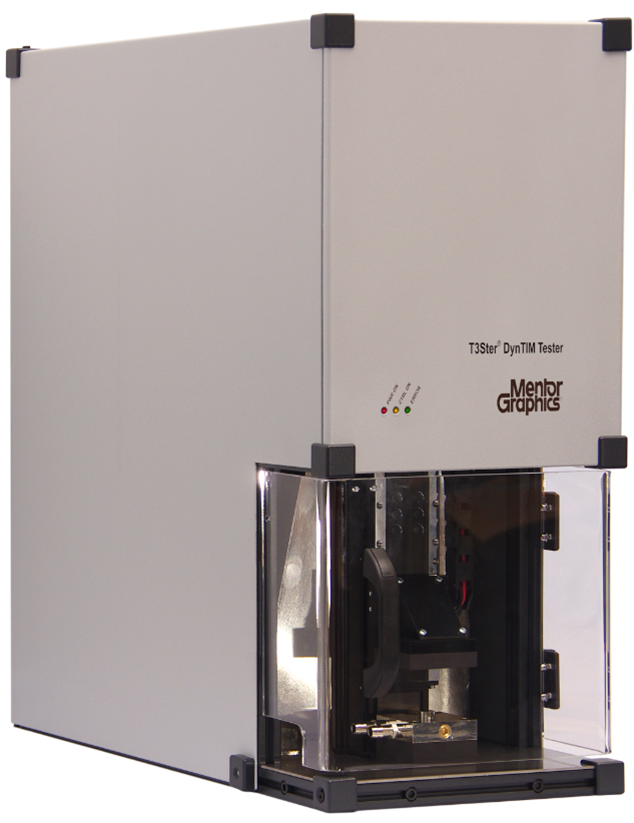 Here at the Mechanical Analysis Division of Mentor we are uniquely placed to provide both experimental test solutions and simulation tools that have been designed to work together to improve the thermal design process. We recently released a hardware product specifically aimed at TIM thermal conductivity measurement, DynTIM. Both a cost effective and highly accurate method of measuring TIM W/mK, it can be employed by an end user to verify or qualify supplier TIM material data or by the supplier themselves to ensure quality spec sheet data is provided to their end users.
Controlling blt (bond line thickness) to an accuracy of a single micron, DynTIM automatically performs a number of thermal resistance measurements on a TIM sample at various blt values. From these measurements the thermal conductivity can be deduced. Here is an example of the range of results that can be obtained…
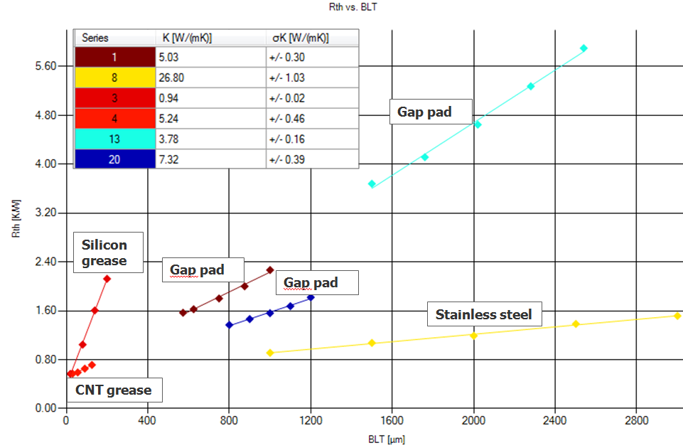
The gradient of the line fit between the Rth vs. blt measurement points is itself the thermal conductivity. TIM development is benefiting from a range of new exotic materials working in combination. The low k CNT (carbon nanotube) grease is a fascinating application of the use of carbon molecules. I’m sure we’ll be seeing much more of carbon nanotubes, graphene sheets etc. in electronics in the future!
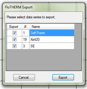 Despite the fact that thermal conductivities are simple single numbers we do also provide a direct interface from DynTIM to FloTHERM that transfers all the deduced conductivities directly to the FloTHERM material attribute library, completely removing the risk of data errors on manual re-entry.
Simulation and experimentation can work well in other ways together, for instance the use of simulation results to explain and support experimental methods as you can see by the use of FloTHERM images in this excellent overview of DynTIM and TIM measurement approaches: http://www.mentor.com/products/mechanical/multimedia/flotherm-tim-webinar
25th January 2013, Ross-on-Wye