By PatMcManus

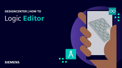
The Logic Editor in Designcenter™ software provides a visual programming environment for several areas of Designcenter.

Algorithmic Modeling gives CAD users a practical way to learn the fundamentals, so it serves as the basis for our example workflow.

There are many existing tutorials showing how to use Algorithmic Modeling to create complex organic shapes, but this article targets new users of the Logic Editor and explains the basic concepts. It starts with basic inputs and math, then builds toward a simple, reusable anti-slip pattern.

If you have created FORTRAN flowcharts on graph paper, documented business use cases in UML or Visio, or worked with low-code tools such as Scratch, Siemens Mendix, or Node-RED then you may already be familiar with Visual programming. Instead of writing low-level code, you connect visual elements that represent inputs, operations, and outputs. In Designcenter, the diagram does more than document the process: it drives the model.

Check out the video below or scroll down to learn more about getting started with the Logic Editor.

Understand the finished example

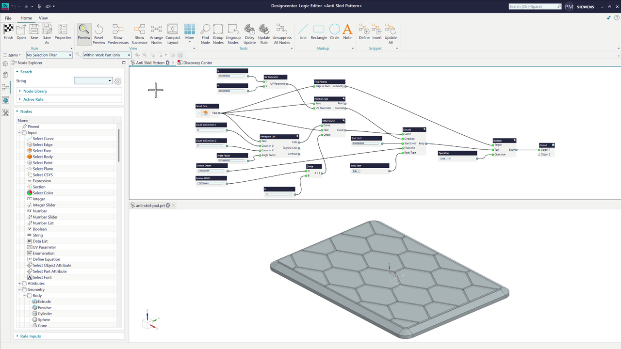
*The finished model will combine simple geometry with a hex pattern, defined by rules defined in the Logic Editor.*

The finished model for this tutorial is a simple anti-fatigue mat. A block with rounded edges and a chamfer forms the base, while an Algorithmic Modeling feature adds a hexagonal anti-slip pattern across the top.

The Logic Editor displays the visual logic above the model. A custom dialog exposes selected values, and changes to those values will update the model according to the rules in the diagram.

Each box in the diagram is a node. Input ports appear on the left, and output ports appear on the right. A node receives data through its input ports, performs an operation, and sends the result through an output port to another node or the final output. Connectors show how data moves through the workflow.

Start with a simple math node

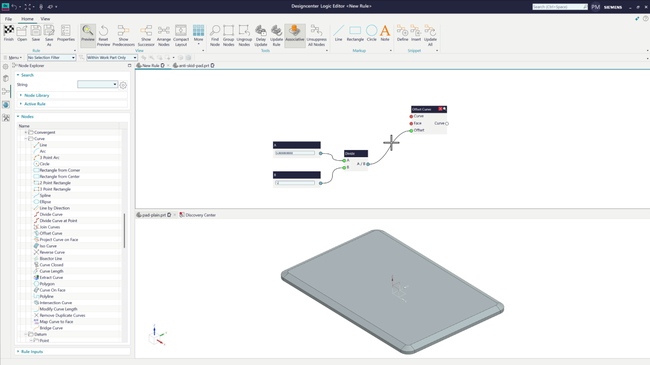
*A simple math node using numbers, like Divide, is easy to understand and nice one to get started with.*

Start with a basic pad shape and add a new Algorithmic Modeling feature. Designcenter opens the Logic Editor above the model and displays the Node Explorer on the left. You can browse nodes by category or search for a specific operation.

An easy way to start is to add a Divide node from the Basic Math category. The node has two inputs, A and B, and one output, A divided by B. Drag in a Number node, connect it to input port A, and let Designcenter generate an appropriate input for B.

The model is live, so it is easy to test the logic with actual values. When A equals 8 and B equals 4, the output equals 2. When A equals 5 and B equals 2, the output equals 2.5. When B equals -2, the output equals -2.5.

This simple example establishes the foundation of the Logic Editor: add nodes, connect them, and pass data from one operation to the next. The rest of the model repeats that same process with additional operations.

Use the result to create geometry

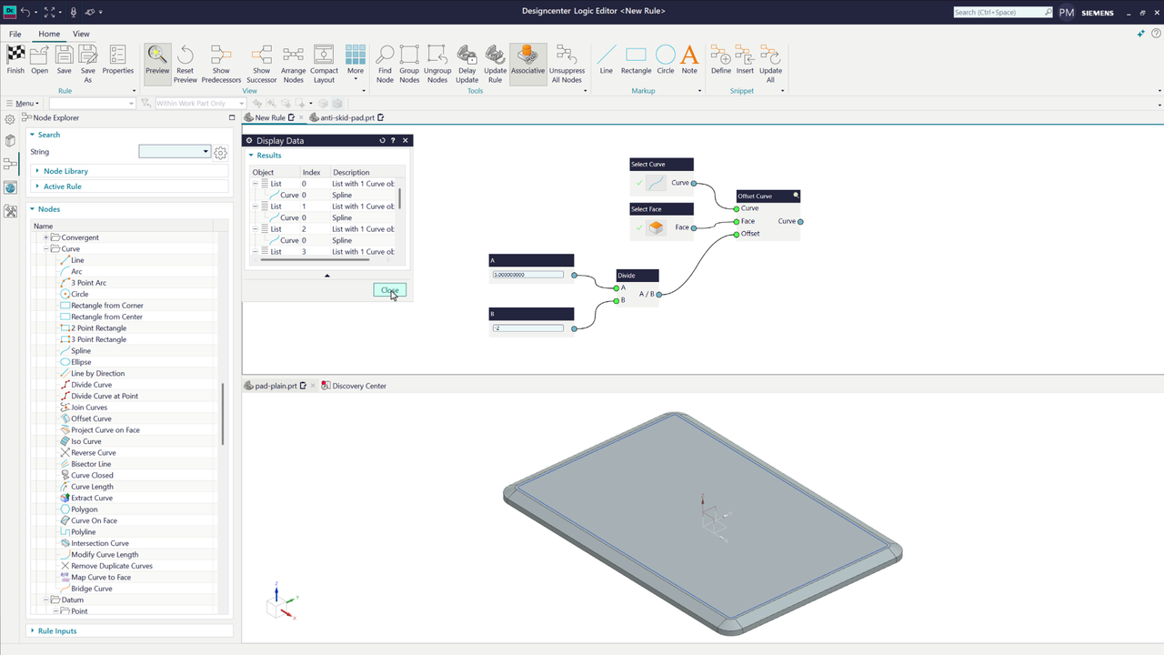
*Getting more complicated by using numbers to create geometry like curves.*

Next, add an Offset Curve node and connect the Divide output as the distance to offset.

The Offset Curve node also requires a face and a set of curves. For an initial test, use the Create Inputs menu to quickly generate two selection nodes.

Select the top face of the pad as the input face, and, for now, select the outer edge loop with Tangent Curves intent as the input curve. We will replace these curves later, but working in small steps makes the logic easier to follow.

Hovering over the ports is an easy way to inspect the data moving through the model. For example, the Offset Curve ports show eight input curves (the four straight sides and four corner blends), each offset by -2.5.

Each node has a Preview toggle for viewing results while you debug. You can also right-click an output port and choose Display Data. Display Data shows the geometry and details for each item in the result. Create an Output node when you want to make a result permanent.

The workflow now combines numerical logic with geometry creation.

Create solid geometry

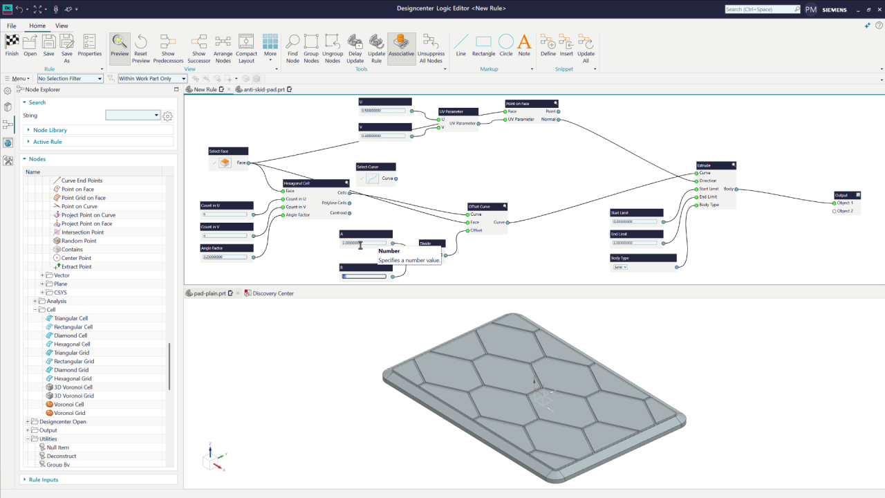
To create solid geometry, add an Extrude node and use the offset curves as its input. Set Body Type to Solid, set the start limit to zero (in the plane of the curves), and temporarily set the end limit (the groove depth) to 5.

The Extrude node also needs a direction. Add a Point on Face node, reuse the selected face as its input, and connect its Normal output to the Extrude Direction port. This node provides both a point on the face and the surface normal at that point.

Set the optional UV location to 0.5, 0.5 so the node consistently uses the center of the face. Explicit values can make the model more robust when the input geometry changes.

Now that the Extrude node works as expected with the outside boundary, replace the temporary boundary curves with a cell pattern to create the anti-slip texture.

Add a Hex Cells node. Use the selected face as the input face, then generate inputs for the U cell count, V cell count, and relative cell size. With both counts set to 10, the preview displays a 10-by-10 hexagonal pattern and a centroid for each cell.

Connect the cell curves to the Offset Curve node in place of the temporary selected curves. The workflow offsets each hexagon inward and passes the result to the Extrude node. Previewing the extrusion shows each hexagon as a solid body. Reduce the cell counts and the extrusion distance until the result matches the intended pattern.

The model still contains separate bodies: one for the pad and one for each hexagon. Add a Boolean node, set its operation to Unite, and use the extruded hexagons as the tool bodies.

The target body already owns the selected face, so the workflow can derive it instead of asking the user to select it again. Add a Find Parents node and reuse the selected face as its input. Because the face is a child of the body, the node returns the body as its parent, so you can use that body as input to Unite.

Confirm that the node returns the correct body in the output preview, then connect it to the Boolean target. The Boolean output becomes the final output of the algorithm.

Clean up the user experience

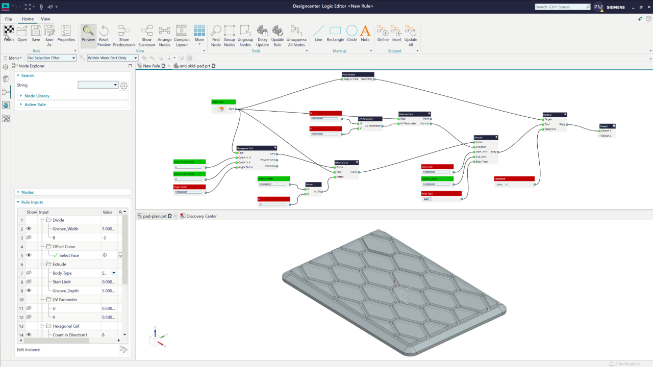
*The logic editor layout and appearance is cleaned up to make it easy to read*

After confirming the model works correctly, remove the temporary Select Curve node and rename the user-facing inputs. Color the user-provided inputs green and the fixed values red to make their use easier to understand. Then arrange the nodes so the data flow remains easy to follow.

The Rule Inputs area uses the renamed nodes to generate the algorithmic feature dialog. Hide any inputs that users do not need to change (the red nodes) so the dialog presents only the controls that matter.

Choose Finish to create the Algorithmic Modeling feature in the part.

To edit the the feature values, double-click the feature in the Part Navigator to open its parameter dialog.

Use Edit Definition if you need to change the underlying rule logic.

You can save the finished Algorithmic Modeling feature to a Reuse Library so you can apply it to other models. When it is time to reuse the Algorithmic Modeling feature, open a new model, locate the feature in the Reuse Library, and drag it into the model. Select the new face, enter the required values, and choose OK. Designcenter creates the patterned geometry in the new model.

Conclusion

This example starts with simple inputs and math, creates and transforms geometry, combines the results into a solid body, exposes only the parameters users need, and saves the finished logic for reuse.

With practice, you can use the Logic Editor to create your own Algorithmic Modeling features or drive other Designcenter commands that use the same visual environment.