Computer Aided Engineering in the Industrial Metaverse – Part 3
The Industrial Metaverse is both a photo- and physics-realistic mirror of reality. A virtual environment where digital twins can be interacted with. From a physical phenomenon perspective, this requires the digital twin to update its behaviour in real-time. This is challenging when considering 3D thermal behaviour as classical methods of thermal 3D simulation fall far short of real-time interactivity requirements. However, thanks to our novel BCI-ROM technology the vision of an interactive Industrial Metaverse is now that much closer to realisation.
Warning: The videos in this blog post may contain flashing imagery not suitable for photo-sensitive audience.
Electronic thermal BCI-ROMs are a gamechanger
Legacy approaches to the thermally simulation of electronic devices were mostly predicated on some kind of abstraction to an equivalent thermal circuit. Even then only a few individual temperature points within the electronic device could be predicted. Subsequent advancements in the mathematical field of Model Order Reduction are now employed in Simcenter Flotherm and Simcenter FLOEFD to be able to author ‘BCI-ROMs’ (Boundary Condition Independent Reduced Order Models). These BCI-ROMs resolve the constraints and restrictions of equivalent thermal circuit models and are capable of simulating the entire transient 3D temperature field of an electronic device, in real-time.
Although the primary motivation in the use of BCI-ROMs is to obfuscate the confidential IP of the design and construction of a packaged semiconductor device, the fact that they are fast to solve also makes them an ideal candidate for Industrial Metaverse deployment.
A generic power inverter application
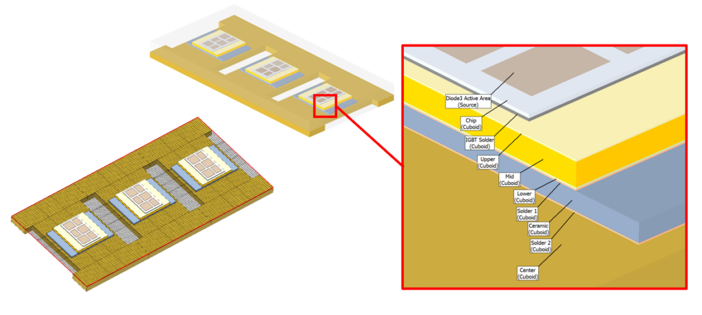
A BCI-ROM is authored from a so called ‘full order model’ (FOM). These full order models are the mainstay of CAE. Starting from a 3D CAD description of the model geometry, material properties are assigned, boundary conditions set (e.g. regions that dissipate thermal power) and then the model is ‘meshed’ (discretised) into many small volumes.
Consider this typical Simcenter Flotherm model of a 3-phase power inverter. Such inverters are used to convert DC into AC to then drive e.g. an electric motor. A fundamental part of an EV e-drive train. For those not familiar with the fundamentals of an inverter, this is a great introduction.
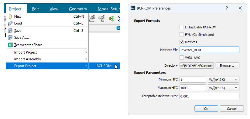
A one-click export option enables the BCI-ROM to be extracted from the FOM and written, in this case, as a series of mathematical matrices in .mtx format.
An NVIDIA Omniverse representation
A digital twin asset in a Metaverse context, such as NVIDIA’s Omniverse, needs to have both a 3D geometric and a physical behaviour representation. Easy enough to take the Simcenter Flotherm geometry and to import that into Omniverse. In Omniverse that geometry is represented as a series of triangular facetted surfaces but visualised as solid rendered surfaces:
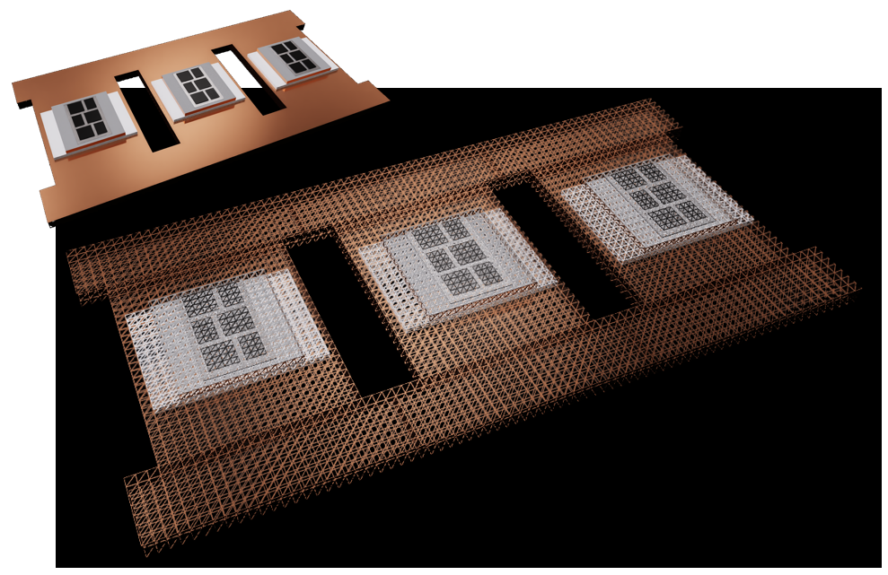
This facetted visualisation representation, although not at the same mesh resolution as the original FOM, is critical for the subsequent rendering of the BCI-ROM temperature results, as well as the time taken to solve and render them without compromising real-time interactivity.
In an industrial metaverse context
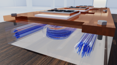
The inverter electronics are then (virtually) placed on a coldplate. This is a block of Aluminium through which water flows, thus convecting the heat away from the electronics above to ensure it does not overheat. This all then placed on a test bench table that sits in a bigger warehouse (though for sure in operation the inverter and coldplate would be installed within an EV).
The coldplate (that is visualised as a glass material part way through the above animation for clarity) is itself pre-simulated using Simcenter FLOEFD to predict the water flow through it. In fact, from this simulation is extracted the resulting HTC (heat transfer coefficient) at the cold plate / inverter interface that is then prescribed when the BCI-ROM of the inverter is subsequently real-time simulated.
A bespoke heads-up-display
Interactivity is enabled via a bespoke HUD that enables control over the absolute level of power dissipation from the 18 semiconductor chips (IGBTs and Diodes). In addition, the ability to change the frequency of power dissipation has been implemented. With a duty cycle of 50% (powered for the half the cycle, off for the other half) the frequency can be adjusted to then see the real-time thermal response.
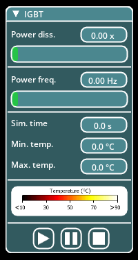
A backend BCI-ROM solver
The .mtx matrices that constitute the BCI-ROM are solved using a standard MATLAB ODE solver (in this case ode15 that has some nice adaptive time stepping capabilities). The absolute power dissipation levels and corresponding frequency is read from the HUD, passed to this backend solver, solved for a time duration, then the results at each point of the surface mesh of the inverter geometry extracted from the BCI-ROM results and then rendered in Omniverse. In all 98592 points are used to query the BCI-ROM with temperature values at each point being returned, converted into a corresponding colour then colour interpolated over the inverter surfaces. This happens automatically, frequently and interactively.
Real-time interactivity
Zero frequency power dissipation
With the frequency set to 0 Hz, the absolute power dissipation can be manually varied via the HUD and the resulting surface temperature response of the inverter geometry visualised in Omniverse (coldplate hidden for clarity).
It’s important to note that the perceived lag between changing the HUD slider-bar power and the resulting thermal response is not a real-time simulation and rendering deficiency, it’s simply the fact that such a system has an inherent physical thermal inertia, or thermal capacitance, where some objects are slower to thermally respond to a change in power than others.
Variable frequency power dissipation
Granted, inverters work normally in the kHz switching frequency range, so fast that it would be near impossible to observe the resulting temperature variations as those switching time scales are much much smaller than the thermal time constants that the system can only respond with.
Is there a limit though on ‘real-time’ simulation? Is there are rate of change of the physics that is soo fast as to not be able to be solved and rendered fast enough? By fixing the absolute power dissipation level in all 18 semiconductor chips, then gradually increasing the frequency of power dissipation we can indeed visually see such a limit:
At some point, in this case at about 7 Hz, we start to see a non-intuitive and non-physical ‘flickering’ of the thermal response. There does indeed come a point where the physics is changing too fast for the solver and renderer to be able to keep pace.
Houston, we have a problem…
A rather technical one for sure, but still.
The attached MATLAB backend ODE solver is called continuously in a threaded way, detached from the rest of the simulation view. The solving time of the MATLAB backend varies somewhere between 20 to 40 milliseconds (ms) when the sliders are untouched. Moving them around has an impact on the attached ODE solver – it has to adapt to the changed inputs. This results in solving times going up to maybe around 100 or even 150 milliseconds for a few (2 to 3 mostly) cycles. This explanation just to give you a feeling of how the results are computed and how long it takes.
Now, if you take a look at the following two figures you see a time scale and diagrams of the frequency applied (“Frequency square wave”). This imposes when power is applied to the model (“Frequency square wave” bigger than 0) and when not (“Frequency square wave” equals 0) – of course depending on the “Power dissipation” slider bar input, which is then used as a factor to the maximum power dissipation. In addition there are vertical lines for each new frame (in gray) and finished MATLAB ODE computations (in red).
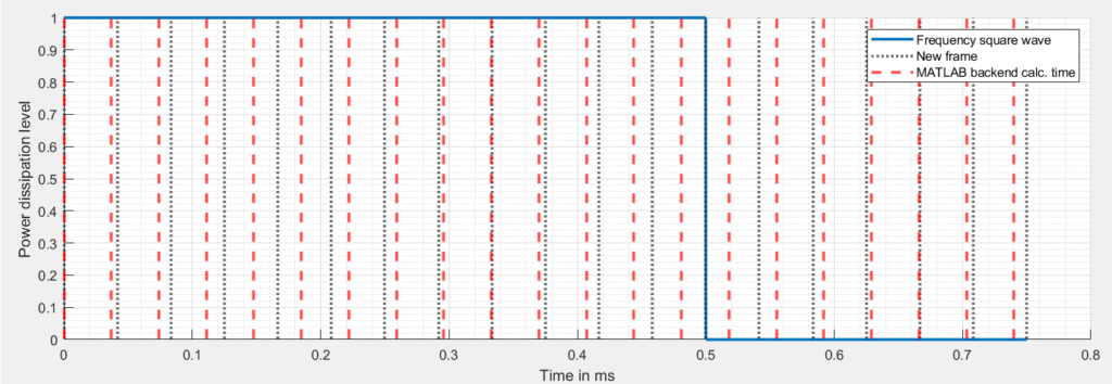
The first figure shows how the system behaves at a frequency of f = 1 hz. Frames and backend computations run along smoothly and even if we miss one frame – nobody can see that.
The second figure (f = 5 hz) shows quite different results.
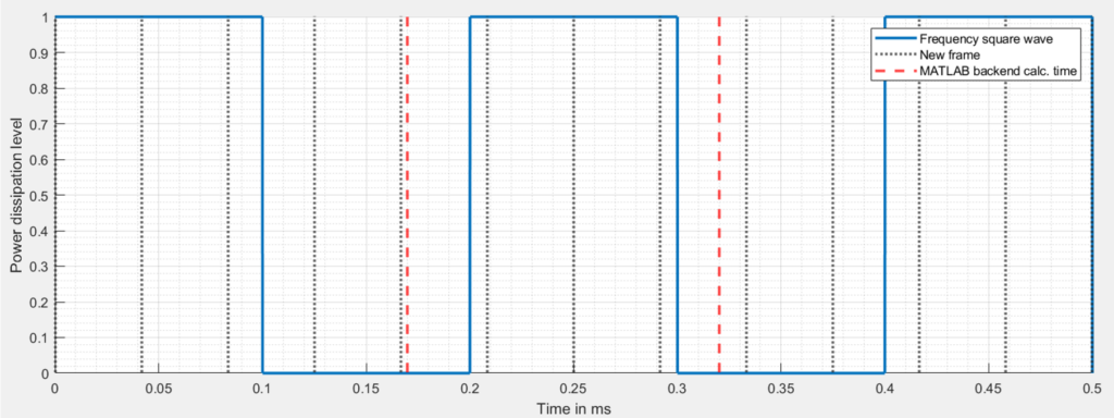
Let’s say the last backend computation stopped (and started) at t=170 ms. This means power dissipation is zero, which will be then communicated to the end user visually. If the next computation takes 150 ms (and stops at t=320 ms), again the resulting power dissipation is zero meaning we missed a whole power-on cycle which was taken into consideration in the attached ODE solver but is not shown to the user.
For our simulation this means that above a frequency setting of around 5 – 10 Hz the visualization will flicker to some extent. This is totally performance dependent of the underlying computer hardware but this border is there – unbreakable. Even if the backend computation would be faster, the next timing border would be the frames per second used to visualize the results.
The interested reader can find more information about the involved Nyquist–Shannon sampling theorem on Wikipedia.
Interactivity without compromising accuracy
There are various ways to create visually compelling, interactive simulation results in real-time, most of which involve some level of compromise on the accuracy of the prediction, or at least require such a long time to extract a real-time model that one might as well just use a FOM instead.
BCI-ROMs are extracted using Krylov sub-space projection methods (plus a whole range of other mathematic refinements). The above BCI-ROM took ~40 minutes to extract from the FOM, didn’t suffer any of the training data requirements that AI/ML approaches necessitate, was extracted to a prescribed accuracy level (in this case ~99%) and can be deployed back within a system level Simcenter Flotherm simulation, solved in Matlab, as VHDL in a Part Quest Explore circuit simulation or even within a 3D Industrial Metaverse context as demonstrated here.
Although these BCI-ROMs just represent thermal conduction applications, their scope for deployment is very wide. AI/ML, despite it’s high profile, isn’t the only way to crack an egg.
- Computer Aided Engineering in the Industrial Metaverse – Part 1
- Computer Aided Engineering in the Industrial Metaverse – Part 2
Disclaimer
This is a research exploration by the Simcenter Technology Innovation team. Our mission: to explore new technologies, to seek out new applications for simulation, and boldly demonstrate the art of the possible where no one has gone before. Therefore, this blog represents only potential product innovations and does not constitute a commitment for delivery. Questions? Contact us at Simcenter_ti.sisw@siemens.com.

Comments
Leave a Reply
You must be logged in to post a comment.
https://skylum.com/blog/dxo-photolab-vs-lightroom qwf