Verification Methodology Reset
Discussion around verification methodologies have been going on for a couple decades. It started back around 2000 with the emergence of the various hardware verification languages (HVLs). Verification specific languages lead to the divergence of design and verification and the creation of the verification engineer. It was HVLs that enabled the transition of directed testing toward constrained random. Early in constrained random adoption it became obvious supporting infrastructure was necessary to be productive; early frameworks included RVM, eRM, AVM, VMM and various homegrown alternatives. The first step in consolidating an approach to constrained random happened with OVM; the final step was UVM which is where we are now.
As time passed and habits formed, UVM became the thing most of us identify with when someone says the word methodology. Constrained random is assumed to be part of that equation being that it’s the workhorse for most teams in our industry. Reuse, also closely associated with methodology, is the primary driver of technical integration with emerging techniques like portable stimulus; UVM, of course, helps form the foundation for that technical integration.
Even if you think beyond UVM, verification methodology radiates from a verification point of view. While born of exploding design complexity, methodologies live solely within verification teams.
Verification_methodology.reset().
I propose reevaluating our current definition of verification methodology. I’d like to see renewed focus on design being the central deliverable and verification methodologies conceived and driven by the needs of design. I’d like to see us break a design into a series of abstractions, identify options for verifying each abstraction, employ techniques best suited to each abstraction and integrate those techniques so transitions are made effectively.
That’s a mouthful. Agree or disagree I think it makes for worthy discussion.
In breaking a design into a set of abstractions, here are five that I identify with: line, block, feature, feature set and system.
A line of code is self explanatory; that’s as low level as it gets. Code block is next; also self explanatory though important to note that code blocks are localized within a design unit (I almost said module there but changed it so I didn’t lose anyone!). Features are where we cross the threshold into characteristics that users identify with yet still don’t provide much value on their own. Simple features will still be localized but more complex features will have a distributed implementation that crosses design unit boundaries. Next are feature sets; definitely distributed across subsystems and the first indication of an actual deliverable. Our highest design abstraction is a complete system where integrated feature sets delivery real-world value.
Examples from each abstraction to help you identify…
- Line: write enable asserted
- Block: write enable pipeline
- Feature: store/load to/from L1 cache
- Feature set: cache coherence
- System: Multicore SoC w/memory subsystem
Identifying options for each abstraction is the fun part of this exercise now that I work for a tool provider. Like I said in Building Integrated Verification Flow – Round 2, I’ve done this before focusing only on simulation techniques due to my own experience being limited to simulation. With Mentor it’s totally different. Suddenly I work with experts that have used all the tools for years and they’re more than happy to share their experience. When you get a cross section of experts sharing their experience, this is what you get…
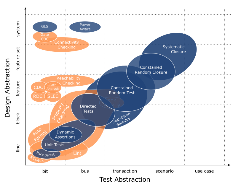
This is a superset of techniques that Mentor provides or enables. Needless to say, there is a lot here (One of my marketing colleagues described it as busy which I’m ok with because it gets the point across that there are a lot of options to consider).
You see I have each technique plotted as design abstraction v. verification abstraction. We already talked about design abstraction; verification abstraction is the level at which we describe interactions in our tests. For example, X-Check is a tool that aims at low level design characteristics (i.e. single line assignments) with properties applied at a bit level; constrained random testing is meant for randomly exercising design features with tests written at a transaction level. And so it goes.
Summarizing why I’ve captured it this way: design abstraction v. test abstraction shows us the sweet spot for a collection of techniques. We see which are best suited to each design abstraction while understanding the test abstraction where they are most effectively applied. The suggestion here is to use tools and techniques within their sweet spot; anywhere else and the value they provide tapers off.
But what’s in all these bubbles? And what do the colours mean?
Good questions. In our next post, I’ll go through each with an explanation and some reasoning for why they are where they are.
-neil
PS: Another reminder that this is work in progress. If you see something you like, something I’m missing, something you disagree with or anything else, please let me know in the comments or send me a note at: neil_johnson@mentor.com.


Comments
Leave a Reply
You must be logged in to post a comment.
Is it just me or is the basis of Constrained Random verification looking a bit shaky?
There are 2 reasons for thinking this:
1- Functional Coverage is just Code Coverage – in a hat.
Lets face it the existence of various state on internal nodes does not indicate a function.
OK, some registers control the mode of operation, but observing them does not mean the function worked correctly.
2- Constrained Random means only using favourable tests
The problem here is the idea of an illegal input combination.
In a safety system, the rule is that all requirements must be verifiable.
An illegal input cannot be verified if constrained out, so a requirement that defines an illegal input is not a requirement.
And what is good policy for a safety system surely applies to all designs.
What we need to say is: if this (bad) input occurs, set a flag.
This is verifiable and opens up the verification space to all combinations.
I agree with David Fitzmaurice. The larger the system, the more activity in the core of the product that will result in high code/functional coverage, yet never actually propagate off-DUT to be visible to the verification system.
Constrained random doesn’t really work for safety-critical systems, because negative testing is implicitly required: you have to make sure that you reject accidentally bad input, and also that you detect and reject malicious input, so you can notify higher levels of the system that you’re under attack. Property checking is the only feasible way of verification when there’s basically an infinite number of possible input stimuli, almost all of which result in the same response (rejection) and only a few that are legal and generate a wide range of responses.
This also leaves out using ‘correct by construction’ tools. if you are able to ensure that your address bus is properly connected, then you don’t need to do constrained random to prove it. The most efficient verification is when none is needed.
I think Property Checking can be greatly expanded, based on what I’ve seen people do with it.
Also, with reuse, verification becomes more of system properties – you’re more watching out for an ’emergent system’ where all the blocks together result in some unexpected behavior. Often it’s bad – deadlocked multiprocessor systems, or a hypercube that’s got its performance in the toilet due to traffic congestion issues between nodes.
An observation about numbers:
20% of a product lifecycle is development,
80% is maintenance.
Of the development phase,
10% definition (specs)
10% DUT coding
80% verification
So the real money savings is in reducing maintenance costs – and that typically means making the DUT easy to test post-production and also easy to upgrade in the field to deal with discovered bugs.
After that, if you do reuse, you will:
1) lowered the cost of verification ( either skip rerunning low-level tests again, or else you do and they all pass), and even if you write the same suite of verification tests, you’ll spend a lot less time isolating failures and then changing the design because you’re ‘correct by construction’.
2) you have both shifted your verification focus from low-level to system-integration level.
And at system level, all the “interesting” functionality that needs verification is in software, not hardware.
I’d like to see IP-XACT or equivalent extended to include system-verification metadata, and a standard on how to use it.
We need to reuse verification IP, just like we reuse RTL IP. An IP “ABC” from vendor XYZ should include the RTL function, timing model, timing constraints, and verification model(s). And then when the user creates instances of ABC, the testbench should be able to be automatically generated.
I’d also include covergroup/coverpoint information in the metadata, so that ABC tells the user when its interfaces have been adequately tested, from the POV of the vendor.
Problems with the constrained random approach to verification.
In constrained random each scenario is constructed more or less at random, and the constraint solver is used to avoid some scenarios, but this clashes with the idea that all requirements must be verifiable.
To see why this is a problem, start by assuming that all requirements must be verifiable. Now let’s say that the requirements document states that certain combinations are not allowed, and can be constrained out. This means that we don’t know what happens in this illegal case. Hence this statement can never be verified, so it cannot be a requirement.
Now assume that it is OK to have a requirement that cannot be verified. Again, the requirements document states that certain combinations are not allowed, and can be constrained out. Again, we don’t know what happens when an illegal case is applied to the inputs. This time the illegal case is part of the requirements, so we cannot discount this case from the functional coverage. This means that if we use constrained random, we never get 100% functional coverage.
In either case we have an incomplete requirements specification, because we don’t know what happens in the illegal case. This is unacceptable as has been established for many years as a cause for concern:
– “The specification may be incomplete in that it does not describe the required behaviour of the system in some critical situation.” (1)
– “Difficulties with requirements are the key root cause of the safety–related software errors which have persisted until integration and system testing.” (2)
(1) Software Engineering (Ian Sommerville, 1995):
(2) Proc. RE 1993 ( Robyn Lutz, 1993)
Either way, the constrained random approach creates a verification problem that cannot be solved. In conclusion, I think it is clear that all requirements, for software or hardware, need to be complete and verifiable, and this means that the constrained random approach to verification is obsolete.
As a guy who worked on this coverage problem for many years at Cadence, good luck, but nice graph and discussion anyway.
One of the problems that faces verification engineers is how to get simulation to play nicely with emulation, given that we are writing UVM testbenches, based on non-synthesisable Verilog code. It looks like the way forward is to move the sequence generation and reference models out of the UVM testbench and into a common scenario generator that can serve both simulation and emulation.
Often when thinking about a problem, it pays to take a different perspective, to get a better insight into the problem, and break out of the dogmatic slumber induced by the (constrained-random) orthodoxy.
This alternative viewpoint is to order tests using the idea of bit distance from a known scenario.
Requirements documents typically describe a scenario and a set of configuration bits that allow variations in behaviour. From this, it is possible to generate all the scenarios that only change one configuration bit.
As these are closely related to the well-known scenario, they should be easy to debug if one fails, since each scenario has got exactly one difference from a well-known scenario.
This is a shallow-first approach to verification, trying all the options that are not too far from a well known scenario. It is also possible to generate a set of scenarios where two of the configuration bits are different from the well-known scenario. There are more of these, but nowhere near the total configuration space that gets sampled using constrained random. This is like exploring the next level of depth, away from the familiar scenario, but if a test needs to be debugged, there are only two differences to look at.
This can go on to any depth, until all the configuration bits are changed. What this is doing is creating a wavefront in configuration space, where each level gets further away from a known scenario.
This approach can help to integrate simulation and emulation flows. For example, shallow tests could be run in simulation and deeper tests in emulation. Test can be shared out like this because instead of using functional coverage, bit distance is the driver. When an emulation test fails, it can be run in simulation for debug, and this is why this scheme needs a common scenario generator and reference model for the two flows.
Also when the expanding wave of scenarios hits a failing test, the run can be terminated to allow for debug. If running all possible scenarios is not realistic, there is a way to decide which tests to set aside; those that are furthest from the normal flow of operations, and pose the least risk to users. Although there is no guarantee that a high bit distance is the same as low risk, it looks like a useful approximation to it.
Since this is a methodical approach to scenario generation, there is a well known formula to calculate the cost of each level, which should help with verification and resource planning.
The number of combinations of N objects taken R at a time is determined by:
C(N,R) = N!/(N−R)!R!
where N is the total number of configuration bits and R is the current bit-distance, the ‘depth’ of the set of scenarios to generate.
If this proposal sounds like a step into the unknown, there is a way to limit it’s risk in use. Normally, a complex IP intended for a system-on-chip application is accompanied by a software release that provides drivers and so on for the customers. This software could provide a routine to measure the bit distance from the list of well-known scenarios of intended usage, and raise a warning flag if the user is going deeper than the verification team went into the depths of the corner cases.
In conclusion, the advantage of this scheme is that it allows us to look at scenario generation from a new perspective, different to constrained random, and not relying on functional coverage. It uses an an ordered rather than random approach and it is in tended to help verification engineers to debug failing tests, by giving a link back to well-known scenarios, the type that get detailed attention in requirements documents.