SerDes Design Part 5: Channel Operating Margin, a Powerful Compliance Tool

In part five of this series about SerDes design, I focus on the adoption and evolution of Channel Operating Margin (COM) as a tool for ensuring compliance of high-speed designs.

First, a History Lesson

Frequency-domain channel performance parameters that were introduced in Annex 69B of the IEEE 802.3ap specification (and later enhanced by other documents), suffered from the lack of trade-offs between various channel impairments. For example, a low-loss channel could tolerate higher insertion loss deviation (ILD), higher crosstalk, or both, but the rigidity of the hard limits did not allow the system designer to make this tradeoff, thus leading to overdesign.

Moreover, the specification did not define any constraint for the reference Tx feed-forward equalization (FFE) and Rx reference equalization that is required for interoperability. This ambiguity forced chip designers to engineer ICs that were more performant than needed in order to avoid possible failures. Over time, it was found that links that met the frequency domain parameters’ limits often failed in the lab. The opposite was also true, links that worked properly on real hardware often failed the specification masks.

The Introduction of COM

In order to overcome the limitations of the compliance flow based on frequency-domain parameters, the industry adopted a new method for some of the protocols operating at 25/28Gbps and higher data rates. This methodology is called Channel Operating Margin (COM) and was introduced in 2014 by the IEEE 802.3bj specification. Described in great detail in Annex 93A of this specification, the mathematical algorithm has its foundation in the statistical signal-processing techniques developed a decade ago.

COM’s mathematical procedure might be intimidating for many people but, from a high-level perspective, COM can be considered similar to a typical statistical simulation. The characteristics of the transmitters and receivers are built into the algorithm. On the transmitter side, the following parameters are included in the simulations:

• Differential peak output voltage for victim and FEXT/NEXT aggressors
• Number of signal levels (two for NRZ modulation and four for PAM4)
• Level separation mismatch
• Random and Dual-Dirac jitter
• One-sided noise spectral density
• Number of FFE taps along with min/max/step constraints for each tap
• Single-ended termination resistance

The receiver model consists of:

• Receiver 3dB bandwidth
• CTLE’s characteristics and constraints such as DC gain, zero and poles frequencies
• DFE length and its normalized coefficient magnitude limit
• Single ended termination resistance

Determining Compliance

Tx and Rx packages are modelled as PI networks consisting of single-ended transmission lines with one capacitor at each end. The value of the two capacitances and the characteristics of the transmission lines are also part of the specification which defines two tests, one for a long package (TL length = 30mm) and another one for a short package (12mm). The long package is required to represent the loss in large packages more susceptible to noise, while the short package is required to interact with reflective channels. The NEXT path always contains a short length package. A channel is compliant only if it passes both tests.

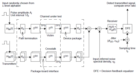
The channel is modelled as a collection of 4-port s-parameter (s4p) files, one for the victim channel and one for each significant aggressor. The maximum number and aggressor types to be included in the simulation are defined not by the specification, but by the user based on the specifics of each design. The COM reference model shown below is a die-to-die representation of the full channel that includes the Tx and Rx models, Tx and Rx terminations, the packages, and the channel.

The Math behind COM Simulations

The mathematical algorithm can be described as a three-step process:

1. Frequency domain (FD) transformations and conversion to time domain (TD)
2. TD signal processing and optimization
3. Final COM calculation

The computational process starts with the channel’s 4-port scattering parameters of the victim path and all the significant, non-alien, crosstalk aggressors, obtained from measurements, electromagnetic simulations, etc. These models are converted to differential mode only, and then cascaded with generic package models and single-ended terminations to obtain the voltage transfer function of the victim and aggressor signal paths. Next, the transmitter feed-forward equalization and receiver continuous-time linear equalization (CTLE) are applied by multiplying the non-equalized transfer functions with FFE and CTLE transfer functions.

The equalized transfer functions are converted into a single-bit response (SBR) by inverse Fast Fourier Transform (IFFT). The SBRs are shaped with an optimized combination of Tx and Rx equalization based on a “full grid search” of the configuration space which is denoted by the minimum reference requirements defined in the standard and a signal-to-noise ratio (SNR) optimization figure of merit (FOM). Noise and jitter are included in the calculation by convoluting their amplitude distribution with that obtained due to intersymbol interference (ISI) and crosstalk.

The final result is a die-to-die figure of merit, defined as the decibel ratio of signal amplitude peak interference to statistical noise amplitude:

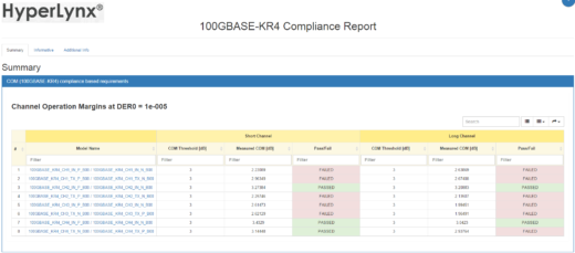
where  is the amplitude of the signal and  is the peak-to-peak amplitude of the noise at the sampling point for a given target detector error ratio (denoted by DER₀). A channel is considered to be compliant if the computed COM value is larger than a specific threshold value, which typically is in the 2dB to 3dB range. This threshold value was included to account for various impairments that are not accounted for in the COM algorithm. An optional, forward error correction (FEC) block can be included in the receive path to identify and correct some bit errors. Channels that include FEC have less stringent requirements for DER₀. An example of a HyperLynx® IEEE COM report for a 100GBASE-KR4 channel is shown below.

What’s Next for COM?

Compared to full statistical simulators, COM was built on several assumptions that were needed to simplify the algorithm and improve its performance. Some areas affected by those simplifications are the computations of the contributions from the input jitter and crosstalk. Moreover, COM considers only two package variations based on long and short transmission line models. It also constrains the fixed FFE architecture to two or three variable tap coefficients and the CTLE implementation to two or three poles and one or two zeros. Some of those limitations are being addressed by JCOM to allow for custom device package and transceiver models to be used jointly with the COM algorithm.

Summary

In its short existence, COM has proven to be flexible, efficient, and easy to use. It was quickly embraced by the engineering community and standardization committee bodies such as OIF-CEI, Fibre Channel, and JEDEC and it continues to evolve, with newer revisions of the specification being released.

For a comparison of COM with statistical eyes, read this DesignCon Best Paper co-authored by Wild River. Also of interest is this six-minute video showing how COM can quickly assess the serial channel performance of an Ethernet backplane.